TLDR: LuenbergerPLL is a C routine designed for tracking sine waves in noisy environments using a particular Luenberger observer.
The LuenbergerPLL routine serves as an efficient tool for tracking sine waves that are subject to various disturbances, providing clean values, amplitude, and phase. It can also be effectively utilized to extract signals in phasor form from measurements.
This problem frequently presents itself in the field of electrical engineering, particularly when working with alternating current (AC). For instance, when voltage or current measurements within an electrical circuit are required.
This repository hosts an implementation of an algorithm that is based on a specific version of the Luenberger observer. I developed this algorithm during my spare time with the goal of creating a tracker that is efficient, robust, easy to use, and simple to tune. All you need to know is the expected frequency of the sine wave and the uncertainty associated with it.
The Derivation section provides a detailed explanation of how this observer is derived. However, please be aware that if you're not familiar with Control Systems and Digital Signal Processing topics, it might be challenging to follow. Regardless, you can bypass that section and directly use the library which is designed to work right out of the box.
The library in this repository consists of two files: LPLL.h which you have to include in your source file and LPLL.c.
In the library, the following structure is defined:
struct LPLL_SS
{
    double A[2][2];
    double B[2];
    double C[2][2];
    double D[2];
};
This struct contains the discrete time filter parameters.
In addition, the library provides the following function:
struct LPLL_SS LPLL_filterDesign(double f0, double BW, double dt);
This function allows you to design a filter taking in as input the expected sine wave frequency $f_0$ in Hz, the filter bandwidth $BW$ in Hz, and the sampling time $dt$ in seconds.
The designed filter is capable of tracking a sine wave based on its measurements. You can choose the bandwidth $BW$ to set an uncertainty level on the sine wave frequency $f_0$. Please note, however, that a narrow bandwidth will require more time for the observer to converge to the sine wave.
Additionally, the library provides the following function:
void LPLL_step(const struct LPLL_SS *ss, double x[], double u, double y[])
This function allows you to filter the signal $u_k$, which is your measurement, and outputs a vector $\underline y$. These are the two outputs of the filter, representing the reconstruction of the two coordinates of a rotating vector generating the wave you are measuring. The 2-element state of the digital filter $\underline x$ must be passed to the filter at each iteration.
The LPLL_step() function is designed to be called at each sampling time, which is every $dt$ seconds, once you have taken your measurement.
To initialize the tracking you should initialize the state vector in an initial state, for example:
double x[2] = { 0.0, 1.0 };
If you are interested in estimating the phase it's advisable to avoid the $(0,0)$ point because $atan2(0,0)$ is not well defined.
You can see the LPLL_test as example.
We begin with the model of a generic vector rotating in the $x_1$, $x_2$ plane with angular speed $\omega$, and amplitude $\rho$:
$$ x_1(t) = \rho \cdot cos(\omega t + \varphi_0) $$
$$ x_2(t) = \rho \cdot sin(\omega t + \varphi_0) $$
We differentiate the state $\underline x$ to obtain an ODE that drives the vector in the plane:
$$ \frac{d}{dt}x_1(t) = -\rho \cdot \omega \cdot sin(\omega t + \varphi_0) = -\omega \cdot x_2(t)$$
$$ \frac{d}{dt}x_2(t) = \rho\cdot \omega \cdot cos(\omega t + \varphi_0) = \omega \cdot x_1(t)$$
In matrix form, defining an output $y$ we can define
$$
\frac{d}{dt}
\begin{bmatrix}
x_1(t) \\
x_2(t)
\end{bmatrix} =
\begin{bmatrix}
0 & -\omega \\
\omega & 0
\end{bmatrix}
\begin{bmatrix}
x_1(t) \\
x_2(t)
\end{bmatrix}
$$
$$
y =
\begin{bmatrix}
1 & 0
\end{bmatrix}
\begin{bmatrix}
x_1(t) \\
x_2(t)
\end{bmatrix}
$$
$$
\begin{matrix}
A_c \triangleq
\begin{bmatrix}
0 & -\omega \\
\omega & 0
\end{bmatrix}
& &
C_c \triangleq
\begin{bmatrix}
1 & 0
\end{bmatrix}
\end{matrix}
$$
Note that the system parameters are independent of the variable $\rho$. The information about this variable is contained within the state $\underline x$.
$$ \rho = \sqrt{x_1^2 + x_2^2} = \sqrt{\underline x^T \underline x} $$
and the instantaneous phase is
$$ \varphi = atan2(x_2, x_1) $$
Now, we can design an observer to estimate the two states. We choose a Luenberger Observer for reasons that will become clear later. We augment the evolution equation with the $L$ gains matrix in order to define the estimated state $\hat{\underline x}(t)$ from the measurement signal $y_m(t)$:
$$ \frac{d}{dt} \hat{\underline x}(t) = A_c \cdot \underline x(t) - L(C_c \hat{\underline x}(t) - y_m(t)) $$
We define the closed loop update matrix
$$ A_{cl} \triangleq A_c - L C $$
To allow the observer to converge we must define a $L$ matrix such that $A_{cl}$ is Hurwitz. Instead of looking for stable eigenvalues we can observe that if we choose an $L$ matrix in the family
$$
L =
\begin{bmatrix}
0
\\
\frac{\omega}{Q}
\end{bmatrix}
$$
for some $Q$, the closed loop matrix becomes:
$$ A_{cl} =
\begin{bmatrix}
0 & -\omega \\
\omega & -\frac{\omega}{Q}
\end{bmatrix}
$$
it can be shown that exists a particular basis where $A_{cl}$ is a state update matrix for a second-order analog bandpass filter with quality factor $Q$. The $A_{cl}$ is Hurwitz because we know from filter theory that the second-order bandpass filter is stable. The quality factor is defined as:
$$ Q \triangleq \frac{f_0}{BW} $$
Where $f_0 = \frac{\omega}{2 \pi}$ and $BW$ is the filter band in $Hz$. So with this $L$ family, the Luenberger observer become a second-order bandpass filter in the coordinate system we initially choose.
This is very useful, meaning we can tune the observer simply by choosing a bandwidth that we can interpret as the uncertainty we have on the central pulsation $\omega$ that we use for the mathematical system model.
The analog filter model will be:
$$ \frac{d}{dt} \hat{\underline x}(t) = A_{cl} \cdot \hat{\underline x}(t) + L\cdot y_m(t) $$
$$ \underline h(t) = C_I \cdot \hat{\underline x}(t) $$
$\underline h(t)$ is the output of the filter. We've defined a SIMO (Single Input Multiple Outputs) filter such that $\underline h(t) = \hat{\underline x}(t)$ so $C_I$ is the identity matrix. This will be useful for the discretization step, which allows us to implement the filter algorithmically.
To obtain good observation performance in the discrete domain, we will discretize the fileter using the Bilinear Transform with prewarping at the $f_0$ frequency. This can be see as a map from Laplace to z-transform domain such that:
$$ s \leftarrow \frac{\omega}{\tan(\omega \Delta T/2)}\cdot\frac{z-1}{z+1} $$
Where $\Delta T$ is the sampling time of the digital system. The prewarping allows the transfer function of the digital filter to match the one of the analog filter at the central frequency $f_0$.
In the matrix state space representation, this transform becomes:
$$
\begin{matrix}
\alpha \triangleq \frac{\omega}{\tan(\omega \Delta T/2)} &
I \triangleq \left(I_d - \frac{1}{\alpha} A_{cl}\right)^{-1}
\end{matrix}
$$
$$
\begin{matrix}
A_d = \left(I_d +\frac{1}{\alpha} A_{cl}\right) I & B_d = \sqrt{\frac{2}{\alpha}} I \cdot L \\
C_d = \sqrt{\frac{2}{\alpha}} C_I I & D_d = D_I +\frac{1}{\alpha} C_I
\end{matrix}
$$
where $I_d$ is the identity matrix and $D_I$ the feed-forward term of the analog filter that is equal to $\underline 0$.
The digital filter equations are
$$ \underline x_{k+1} = A_d \cdot \underline x_k + B_d \cdot {y_m}_k $$
$$ \underline h_k = C_d \cdot \underline x_k + D_d \cdot {y_m}_k $$
The reconstruction of the state of the rotating vector at the instant $k$ will be the $\underline h_k$ vector.
otavePlotter.m provides an Octave script to plot the output of LPLL_test:
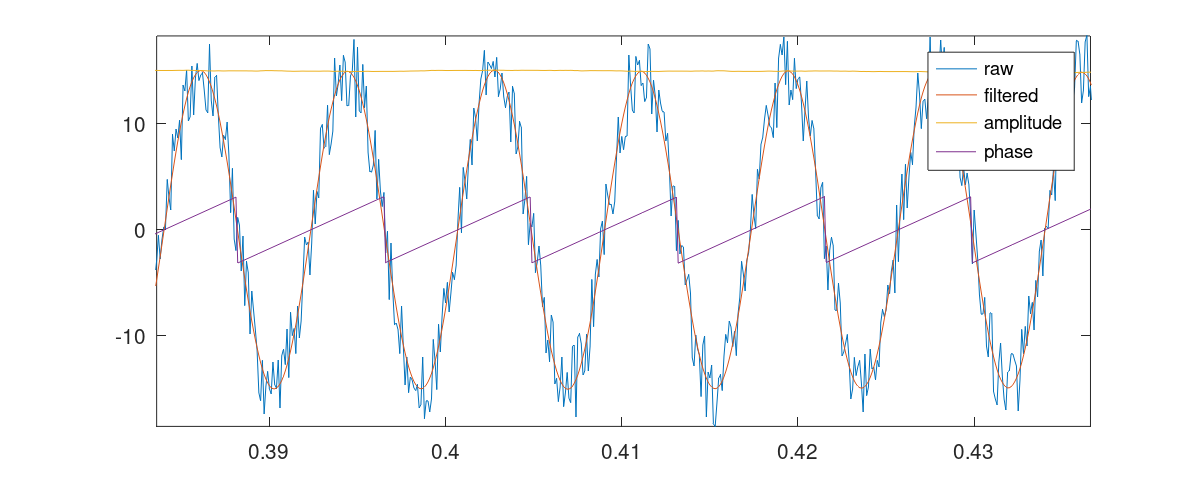
You can see that the observer converge to the sine wave and allow you to estimate the cleaned sin wave, the amplitude $\rho$ and the instantaneous phase.
In a steady-state circuit analysis using the Steinmetz transform, it's common to convert time domain sine wave signals in phasor form:
$$
\rho \cdot cos(\omega t + \varphi_0) \rightarrow \frac{\rho}{\sqrt 2} e^{j \varphi_0}
$$
The LPLL filter allows you to estimate phasors. In fact you can derive $\rho$ as
$$ \rho = \sqrt{\underline h^T \underline h} $$
However, you don't know the initial phase $\varphi_0$. What you really need is the phase displacement of signals. Hence, you need to choose a reference system for the phases, forcing a signal to have $\varphi_0 = 0$. Then, you can easily calculate the phase displacement from the reference signal using the following trigonometric identity:
$$
tan(a - b) = \frac{sin(a) cos(b) - cos(a) sin(b)}{sin(a) sin(b) + cos(a)cos(b)}
$$
If we have two signals and one of the previous filter for each signal, we get a pair $\underline h_1$ and $\underline h_2$ of outputs.
When the identity is applied to the filter output, we obtain
$$
\frac{{h_2}_2 {h_1}_1 - {h_2}_1 {h_1}_2}{{h_2}_1 {h_1}_1 - {h_2}_2 {h_1}_2} =
\frac{\rho_1 \rho_2}{\rho_1 \rho_2} tan(\varphi_2 - \varphi_1) =
tan(\varphi_2 - \varphi_1)
$$
Thus, we can observe that
$$
\Delta \varphi = atan2({h_2}_2 {h_1}_1 - {h_2}_1 {h_1}_2, {h_2}_1 {h_1}_1 - {h_2}_2 {h_1}_2)
$$
The phasor form of the two signals will then be
$$ F_1 = \frac{\rho_1}{\sqrt 2}e^{j0} = \frac{\rho_1}{\sqrt 2} $$
$$ F_2 = \frac{\rho_2}{\sqrt 2}e^{j \Delta \varphi} $$
