amf71 / cloneMap

An R package to plot maps of clone distributions in somatic evolution

cloneMap

Description

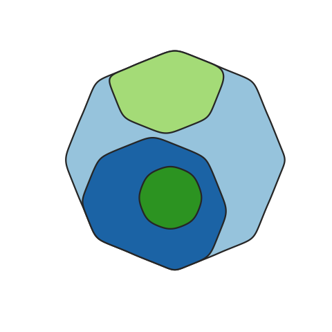
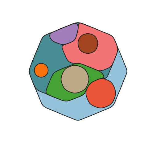
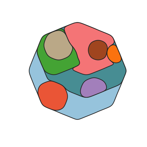
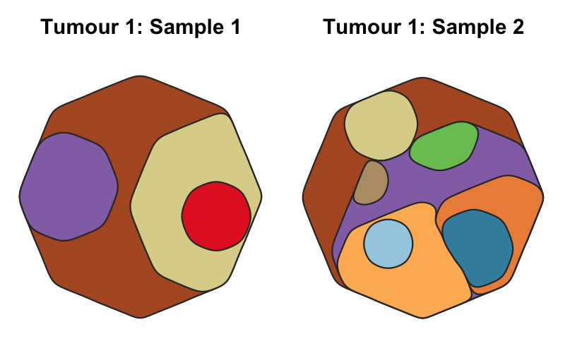
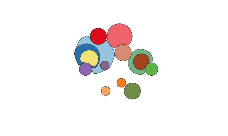
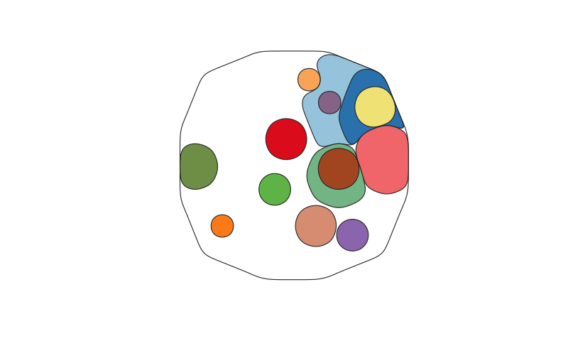
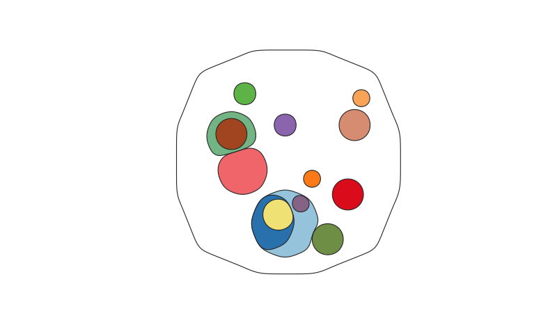
A function to map the distribution of somatic clones in sample or set of samples, accounting for the clone size(s), ie the Cancer Cell Fraction (CCF), and phylogenetic relationships between clones. Clone positions are semi-randomised in the plot while maintaining the two formally described factors.

Installation & loading

Unfortunately the R package Rgeos which is required for cloneMaps has been archieved on CRAN. Therefore install geos using homebrew and install the R package using R-Forge:

brew install geos

install.packages("rgeos", repos="http://R-Forge.R-project.org", type="source”)

You can then use devtools::install_github() to install cloneMap from this repository:

devtools::install_github("amf71/cloneMap")`

load package:

library(cloneMap)

Usage examples - rooted trees

Example data

tree_example_1, tree_example_2, tree_example, CCFs_example_1, CCFs_example_2, and clone_colours_example are loaded into the R environment (hidden) upon package loading and also are defined below:

Example CCF tables, these could be from the same tumour

CCFs_example_1 <- data.frame( clones = c( 1,   2,   3,   4 ), 
                              CCF    = c( 1, 0.4, 0.2, 0.1 ), 
                              stringsAsFactors = F)

CCFs_example_2 <- data.frame( clones = c( 1,   2,   3,   5,    6,    7,    8,   9,   10 ), 
                              CCF    = c( 1, 0.1, 0.7, 0.2, 0.25, 0.03, 0.06, 0.1, 0.05 ), 
                              stringsAsFactors = F )

Example tree matricies are written with each relationship as a row, the parent as the first column and child as the second

tree_example_1  <-  matrix( c(1, 2,
                              1, 3,
                              2, 4 ), ncol = 2, byrow = TRUE )

tree_example_2  <-  matrix( c(1, 2,
                              1, 3,
                              3, 5,
                              3, 6,
                              3, 7,
                              3, 8,
                              5, 9, 
                              6, 10 ), ncol = 2, byrow = TRUE )

tree_example   <-   matrix( c(1, 2,
                              1, 3,
                              2, 4,
                              3, 5,
                              3, 6,
                              3, 7,
                              3, 8,
                              5, 9, 
                              6, 10 ), ncol = 2, byrow = TRUE )

Example colours are define using a named vector of hexidecimal colours with clones as names

clone.names <- unique( c( tree_example[,1], tree_example[,2] ) )

clone_colours_example <- c( "#B15928", "#DDD399", "#9471B4", "#ED8F47", "#FDB762", 
                            "#E52829", "#B89B74", "#79C360", "#3F8EAA", "#A6CEE3" ) 

names(clone_colours_example) <- clone.names

Additionally a function is provided to make clone colour input objects using a specified RColourBrewer pallete (default = "Paired" palette)

clone.names <- unique( c( tree_example[,1], tree_example[,2] ) )

clone_colours_example_2 <- make_clone_col_input( clone.names )

Plot examples

Simple map:

cloneMap( tree_example_1, CCFs_example_1 )

More complex map:

cloneMap( tree_example_2, CCFs_example_2 )

Use a clone_map object to plot cloneMaps reproducably and much faster:

clone_map_eg <- cloneMap( tree_example_2, CCFs_example_2, output.Clone.map.obj = TRUE, plot.data = FALSE )
cloneMap( clone_map = clone_map_eg )

Specify the same clone colours accross several plots:

cloneMap( tree_example, CCFs_example_1, clone.cols = clone_colours_example )
cloneMap( tree_example, CCFs_example_2, clone.cols = clone_colours_example )

Usage examples - unrooted trees

cloneMaps will also plot unrooted trees - i.e. where some clones are not related to each other. This is common in data derived from normal tissues, rather than tumours, which are dominated by small unrelated clones.

If a clone has no parents or daughters it is specified as clone name (parent) -> clone name (child) as for clones 1, 2, 9, 10, 11, 12, 13 and 14 in the example below.

Example data

tree_example_poly, CCF_example_poly are loaded into the R environment (hidden) upon package loading and also are defined below:

Example CCF table for unrooted data

CCF_example_poly <- data.frame( clones = c( 1,   2,    3,   4,    5,    6,    7,    8,    9,   10,     11,   12,    13,   14 ), 
                                CCF    = c( 0.03, 0.05, 0.2, 0.1, 0.02, 0.05,  0.1,  0.05, 0.1, 0.05, 0.02, 0.02, 0.05, 0.03 ), 
                                stringsAsFactors = F )

Example tree matrix for unrooted data. Each relationship is specified as a row, the parent as the first column and child as the second

tree_example_poly <-   matrix( c(1, 1,
                                 2, 2,
                                 3, 4,
                                 3, 5,
                                 4, 6,
                                 7, 8,
                                 9, 9,
                                 10, 10,
                                 11, 11,
                                 12, 12,
                                 13, 13,
                                 14, 14), ncol = 2, byrow = TRUE )

Plot examples

Plot map of polyclonal data similar to that found in normal tissues.

cloneMap( tree.mat = tree_example_poly, 
          CCF.data = CCF_example_poly )

Plot map of polyclonal data similar to that found in normal tissues with border around the plot area. This makes clearer the % of the tissue containing mutant clones.

cloneMap( tree.mat = tree_example_poly, 
          CCF.data = CCF_example_poly,
          tissue_border = TRUE)

Plot map of polyclonal data similar to that found in normal tissues with border with sparsely spaced clones. Here space_fraction indicates that 70% of the plot area should be white space indicating that only 70% of cells are wildtype.

cloneMap( tree.mat = tree_example_poly, 
          CCF.data = CCF_example_poly,
          tissue_border = TRUE,
          space_fraction = 0.7 )