In a nutshell, the goal of this project is to create an rnnlm implementation that can be trained on huge datasets (several billions of words) and very large vocabularies (several hundred thousands) and used in real-world ASR and MT problems. Besides, to achieve better results this implementation supports such praised setups as ReLU+DiagonalInitialization [1], GRU [2], NCE [3], and RMSProp [4].
How fast is it? Well, on One Billion Word Benchmark [8] and 3.3GHz CPU the program with standard parameters (sigmoid hidden layer of size 256 and hierarchical softmax) processes more then 250k words per second in 8 threads, i.e. 15 millions of words per minute. As a result an epoch takes less than one hour. Check Experiments section for more numbers and figures.
The distribution includes ./run_benchmark.sh script to compare training speed on your machine among several implementations.
The scripts downloads Penn Tree Bank corpus and trains four models: Mikolov's rnnlm with class-based softmax from here, Edrenkin's rnnlm with HS from Kaldi project, faster-rnnlm with hierarchical softmax, and faster-rnnlm with noise contrastive estimation.
Note that while models with class-based softmax can achieve a little lower entropy then models hierarchical softmax, their training is infeasible for large vocabularies.
On the other hand, NCE speed doesn't depend on the size of the vocabulary.
Whats more, models trained with NCE is comparable with class-based models in terms of resulting entropy.
Run ./build.sh to download Eigen library and build faster-rnnlm.
To train a simple model with GRU hidden unit and Noise Contrastive Estimation, use the following command:
./rnnlm -rnnlm model_name -train train.txt -valid validation.txt -hidden 128 -hidden-type gru -nce 20 -alpha 0.01
Files train.txt and test.txt must contain one sentence per line. All distinct words that are found in the training file will be used for the nnet vocab, their counts will determine Huffman tree structure and remain fixed for this nnet. If you prefer using limited vocabulary (say, top 1 million words) you should map all other words to or another token of your choice. Limited vocabulary is usually a good idea if it helps you to have enough training examples for each word.
To apply the model use following command:
./rnnlm -rnnlm model_name -test train.txt
Logprobs (log10) of each sentence are printed to stdout. Entropy of the corpus in bits is printed to stderr.
The neural network has an input embedding layer, a few hidden layers, an output layer, and optional direct input-output connections.
Hidden layer
At the moment the following hidden layers are supported: sigmoid, tanh, relu, gru, gru-bias, gru-insyn, gru-full. First three types are quite standard. Last four types stand for different modification of Gated Recurrent Unit. Namely, gru-insyn follows formulas from [2]; gru-full adds bias terms for reset and update gates; gru uses identity matrices for input transformation without bias; gru-bias is gru with bias terms. The fastest layer is relu, the slowest one is gru-full.
Standard output layer for classification problems is softmax. However, as softmax outputs must be normalized, i.e. sum over all classes must be one, its calculation is infeasible for a very large vocabulary. To overcome this problem one can use either softmax factorization or implicit normalization. By default, we approximate softmax via Hierarchical Softmax over Huffman Tree [6]. It allows to calculate softmax in logarithmic linear time, but reduces the quality of the model. Implicit normalization means that one calculates next word probability as in full softmax case, but without explicit normalization over all the words. Of course, it is not guaranteed that such probabilities will sum to up. But in practice the sum is quite close to one due to custom loss function. Checkout [3] for more details.
As was noted in [0], simultaneous training of neural network together with maximum entropy model could lead to significant improvement. In a nutshell, maxent model tries to approximate probability of target as a linear combination of its history features. E.g. in order to estimate probability if word "d" in the sentence "a b c d", the model will sum the following features: f("d") + f("c d") + f("b c d") + f("a b c d"). You can use maxent with both HS and NCE output layers.
We provide results of model evaluation on two popular datasets: PTB and One Billion Word Benchmark. Checkout doc/RESULTS.md for reasonable parameters.
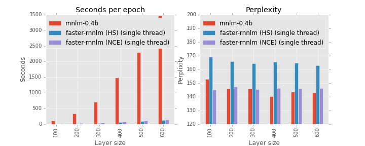
The most popular corpus for LM benchmarks is English Penn Treebank. Its train part contains a little less than 1kk words and the size of vocabulary is 10k words. In other words, it's akin to Iris flower dataset. The size of vocabulary allows one to use less efficient softmax approximation. We compare faster-rnnlm with the latest version of rnnlm toolkit from here. As expected, class-based works a little better than hierarchical softmax, but it is much slower. On the other hand, perplexity for NCE and class-based softmax is comparable while training time differs significantly. What's more, training speed for class-based softmax will decrease with an increase in the size of the vocabulary, while NCE doesn't bother about it. (At least, in theory; in practice, bigger vocabulary will probably increase cache miss frequency.) For fair speed comparison we use only one thread for faster-rnnlm.
Note. We use the following setting: learning_rate = 0.1, noise_samples=30 (for nce), bptt=32+8, threads=1 (for faster-rnnlm).
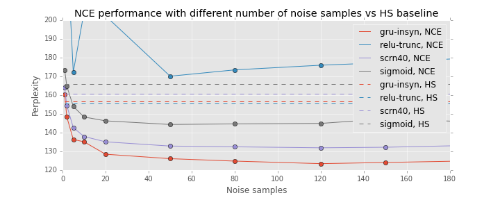
It was shown that RNN models with sigmoid activation functions trained with NCE criterion outperforms ones trained with CE criterion over approximated softmax (e.g. [3]). We tried to reproduce this improvements using other popular architectures, namely, truncated ReLU, Structurally Constrained Recurrent Network [9] with 40 context units, and Gated Recurrent Unit [2]. Surprisingly, not all types of hidden units benefit from NCE. Truncated ReLU achieves the lowest perplexity among all the other units during CE training, and the highest - during NCE training. We used truncated ReLU as standard ReLU works even worse. "Smart" units (SCRN and GRU) demonstrate superior results.
Note. We report the best perplexity after grid search using the following parameters: learning_rate = {0.01, 0.03, 0.1, 0.3, 1.0}, noise_samples = {10, 20, 60} (for nce only), bptt={32+8, 1+8}, diagonal_initialization={None, 0.1, 0.5, 0.9, 1.0}, L2 = {1e-5, 1e-6, 0}.

The following figure shows dependency between number of noise samples and final perplexity for different types of units. Dashed lines indicate perplexity for models with Hierarchical Softmax. It's easy to see that the samples used, the lower the final perplexity is. However, even 5 samples is enough for NCE to work better than HS. Except for relu-trunc, thas couldn't be trained with NCE for any number of noise samples.
Note. We report the best perplexity after grid search. The size of the hidden layer is 200.
For One Billion Word Benchmark we use setup as is it was described in [8] using official scripts. Around 0.8 billion words in the training corpus; 793471 words in the vocabulary (including <s> and </s> words). We use heldout-00000 for validation, and heldout-00001 for testing.
Hierarchical softmax versus Noise Contrastive Estimation. In a nutshell, for bigger vocabularies drawbacks of HS become more significant. As a result, NCE training results in much smaller values of perplexity. It's easy to see that performance of Truncated ReLU on this dataset agrees with experiments on PTB. Namely, RNN with Truncated ReLU units could be training more efficiently with CE, if the layer size is small. However, relative performance of the other unit types have changed. In contrast to PTB experiments, on One Billion Words corpus the simplest unit achieves the best quality.
Note. We report the best perplexity on heldout-00001 after grid search over the learning_rate, bptt, and diagonal_initialization. We use 50 noise samples for NCE training.

The following graph demonstrates dependency between number of noise samples and final perplexity.
Just as in the case of PTB, 5 samples is enough for NCE to significantly outperform NCE.

One important property of RNNLM models is that they are complementary to standard N-gram LM. One way to achieve this is to train maxent model as a part of the neural network mode. That could be achieved by --direct and --direct-order options. Another way to achieve the same effect is to use external language model. We use Interpolated KN 5-gram model that is shipped with the benchmark.
Maxent model significantly decrease perplexity for all hidden layer types and sizes. Moreover, it diminishes the impact of layer size. As expected, combination of RNNLM-ME and KN works better than any of them (perplexity of the KN model is 73).
Note. We took the best performing models from the previous and added maxent layer of size 1000 and order 3.

We opted to use command line options that are compatible with Mikolov's rnnlm. As result one can just replace the binary to switch between implementations.
The program has three modes, i.e. training, evaluation, and sampling.
All modes require model name:
    --rnnlm <file>
      Path to model file
Will create and .nnet files (for storing vocab/counts in the text form and the net itself in binary form). If the and .nnet already exist, the tool will attempt to load them instead of starting new training. If the exists and .nnet doesn't, the tool will use existing vocabulary and new weights.
To run program in test mode, you must provide test file. If you use NCE and would like to calculate entropy, you must use --nce_accurate_test flag. All other options are ignored in apply mode
    --test <file>
      Test file
    --nce-accurate-test (0 | 1)
      Explicitly normalize output probabilities; use this option
      to compute actual entropy (default: 0)
To run program in sampling mode, you must select positive number of sentences to sample.
  --generate-samples <int>
    Number of sentences to generate in sampling mode (default: 0)
  --generate-temperature <float>
    Softmax temperature (use lower values to get robuster results) (default: 1)
To train program, you must provide train and validation files
  --train <file>
    Train file
  --valid <file>
    Validation file (used for early stopping)
Model structure options
  --hidden <int>
    Size of embedding and hidden layers (default: 100)
  --hidden-type <string>
    Hidden layer activation (sigmoid, tanh, relu, gru, gru-bias, gru-insyn, gru-full)
    (default: sigmoid)
  --hidden-count <int>
    Count of hidden layers; all hidden layers have the same type and size (default: 1)
  --arity <int>
    Arity of the HS tree; for HS mode only (default: 2)
  --direct <int>
    Size of maxent layer in millions (default: 0)
  --direct-order <int>
    Maximum order of ngram features (default: 0)
Learning reverse model, i.e. a model that predicts words from last one to first one, could be useful for mixture.
  --reverse-sentence (0 | 1)
    Predict sentence words in reversed order (default: 0)
The performance does not scale linearly with the number of threads (it is sub-linear due to cache misses, false HogWild assumptions, etc). Testing, validation and sampling are always performed by a single thread regardless of this setting. Also checkout "Performance notes" section
  --threads <int>
    Number of threads to use
By default, recurrent weights are initialized using uniform distribution. In [1] another method to initialize weights was suggested, i.e. identity matrix multiplied by some positive constant. The option below corresponds to this constant.
  --diagonal-initialization <float>
    Initialize recurrent matrix with x * I (x is the value and I is identity matrix)
    Must be greater then zero to have any effect (default: 0)
Optimization options
  --rmsprop <float>
    RMSprop coefficient; rmsprop=1 disables rmsprop and rmsprop=0 equivalent to RMS
    (default: 1)
  --gradient-clipping <float>
    Clip updates above the value (default: 1)
  --learn-recurrent (0 | 1)
    Learn hidden layer weights (default: 1)
  --learn-embeddings (0 | 1)
    Learn embedding weights (default: 1)
  --alpha <float>
    Learning rate for recurrent and embedding weights (default: 0.1)
  --maxent-alpha <float>
    Learning rate for maxent layer (default: 0.1)
  --beta <float>
    Weight decay for recurrent and embedding weight, i.e. L2-regularization
    (default: 1e-06)
  --maxent-beta <float>
    Weight decay for maxent layer, i.e. L2-regularization (default: 1e-06)
The program supports truncated back propagation through time. Gradients from hidden to input are back propagated on each time step. However gradients from hidden to previous hidden are propagated for bptt steps within each bppt-period block. This trick could speed up training and wrestle gradient explosion. See [7] for details. To disable any truncation set bptt to zero.
  --bptt <int>
    Length of truncated BPTT unfolding
    Set to zero to back-propagate through entire sentence (default: 3)
  --bptt-skip <int>
    Number of steps without BPTT;
    Doesn't have any effect if bptt is 0 (default: 10)
Early stopping options (see [0]). Let `ratio' be a ratio of previous epoch validation entropy to new one.
  --stop <float>
    If `ratio' less than `stop' then start leaning rate decay (default: 1.003)
  --lr-decay-factor <float>
    Learning rate decay factor (default: 2)
  --reject-threshold <float>
    If (whats more) `ratio' less than `reject-threshold' then purge the epoch
    (default: 0.997)
  --retry <int>
    Stop training once `ratio' has hit `stop' at least `retry' times (default: 2)
Noise Contrastive Estimation is used iff number of noise samples (--nce option) is greater then zero. Otherwise HS is used. Reasonable value for nce is 20.
  --nce <int>
    Number of noise samples; if nce is position then NCE is used instead of HS
    (default: 0)
  --use-cuda (0 | 1)
    Use CUDA to compute validation entropy and test entropy in accurate mode,
    i.e. if nce-accurate-test is true (default: 0)
  --use-cuda-memory-efficient (0 | 1)
    Do not copy the whole maxent layer on GPU. Slower, but could be useful to deal with huge
    maxent layers (default: 0)
  --nce-unigram-power <float>
    Discount power for unigram frequency (default: 1)
  --nce-lnz <float>
    Ln of normalization constant (default: 9)
  --nce-unigram-min-cells <float>
    Minimum number of cells for each word in unigram table (works
    akin to Laplacian smoothing) (default: 5)
  --nce-maxent-model <string>
    Use given the model as a noise generator
    The model must a pure maxent model trained by the program (default: )
Other options
  --epoch-per-file <int>
    Treat one pass over the train file as given number of epochs (default: 1)
  --seed <int>
    Random seed for weight initialization and sampling (default: 0)
  --show-progress (0 | 1)
    Show training progress (default: 1)
  --show-train-entropy (0 | 1)
    Show average entropy on train set for the first thread (default: 0)
    Train entropy calculation doesn't work for NCE
To speed up matrix operations we use Eigen (C++ template library for linear algebra).
Besides, we use data parallelism with sentence-batch HogWild [5].
The best performance could be achieved if all the threads are binded to the same CPU (one thread per core). This could be done by means of taskset tool (available by default in most Linux distros).
E.g. if you have 2 CPUs and each CPU has 8 real cores + 8 hyper threading cores, you should use the following command:
taskset -c 0,1,2,3,4,5,6,7 ./rnnlm -threads 8 ...
In NCE mode CUDA is used to accelerate validation entropy calculation. Of course, if you don't have GPU, you can use CPU to calculate entropy, but it will take a lot of time.
- You don't need to repeat structural parameters (hidden, hidden-type, reverse, direct, direct-order) when using an existing model. They will be ignored. The vocabulary saved in the model will be reused.
- The vocabulary is built based on the training file on the first run of the tool for a particular model. The program will ignore sentences with OOVs in train time (or report them in test time).
- Vocabulary size plays very small role in the performance (it is logarithmic in the size of vocabulary due to the Huffman tree decomposition). Hidden layer size and the amount of training data are the main factors.
- Usually NCE works better then HS in terms of both PPL and WER.
- Direct connections could dramatically improve model quality. Especially in case of HS. Reasonable values to start from are
-direct 1000 -direct-order 4. - The model will be written to file after a training epoch if and only if its validation entropy improved compared to the previous epoch.
- It is a good idea to shuffle sentences in the set before splitting them into training and validation sets (GNU shuf & split are one of the possible choices to do it). For huge datasets use --epoch-per-file option.
[0] Mikolov, T. (2012). Statistical language models based on neural networks. Presentation at Google, Mountain View, 2nd April.
[1] Le, Q. V., Jaitly, N., & Hinton, G. E. (2015). A Simple Way to Initialize Recurrent Networks of Rectified Linear Units. arXiv preprint arXiv:1504.00941.
[2] Chung, J., Gulcehre, C., Cho, K., & Bengio, Y. (2014). Empirical evaluation of gated recurrent neural networks on sequence modeling. arXiv preprint arXiv:1412.3555.
[3] Chen, X., Liu, X., Gales, M. J. F., & Woodland, P. C. (2015). Recurrent neural network language model training with noise contrastive estimation for speech recognition.
[4] T. Tieleman and G. Hinton, “Lecture 6.5-rmsprop: Divide the gradient by a running average of its recent magnitude,” COURSERA: Neural Networks for Machine Learning, vol. 4, 2012
[5] Recht, B., Re, C., Wright, S., & Niu, F. (2011). Hogwild: A lock-free approach to parallelizing stochastic gradient descent. In Advances in Neural Information Processing Systems (pp. 693-701). Chicago
[6] Mikolov, T., Chen, K., Corrado, G., & Dean, J. (2013). Efficient estimation of word representations in vector space. arXiv preprint arXiv:1301.3781.
[7] Sutskever, I. (2013). Training recurrent neural networks (Doctoral dissertation, University of Toronto).
[8] Chelba, C., Mikolov, T., Schuster, M., Ge, Q., Brants, T., Koehn, P., & Robinson, T. (2013). One billion word benchmark for measuring progress in statistical language modeling. arXiv preprint arXiv:1312.3005. GitHub
[9] Mikolov, T., Joulin, A., Chopra, S., Mathieu, M., & Ranzato, M. A. (2014). Learning longer memory in recurrent neural networks. arXiv preprint arXiv:1412.7753.