**Import libraries **
import json
import matplotlib.pyplot as plt
import numpy as np
import pandas as pd

from sklearn.ensemble import RandomForestRegressor
from sklearn.model_selection import cross_val_score
from sklearn.model_selection import train_test_split
from xgboost import XGBRegressor
Download weather data
!wget https://datacases.s3.us-east-2.amazonaws.com/datathon-2020/Ernst+and+Young/Dubai+Weather_20180101_20200316.txt--2020-05-17 11:35:08-- https://datacases.s3.us-east-2.amazonaws.com/datathon-2020/Ernst+and+Young/Dubai+Weather_20180101_20200316.txt
Resolving datacases.s3.us-east-2.amazonaws.com (datacases.s3.us-east-2.amazonaws.com)... 52.219.105.74
Connecting to datacases.s3.us-east-2.amazonaws.com (datacases.s3.us-east-2.amazonaws.com)|52.219.105.74|:443... connected.
HTTP request sent, awaiting response... 200 OK
Length: 6915588 (6.6M) [text/plain]
Saving to: ‘Dubai+Weather_20180101_20200316.txt’
Dubai+Weather_20180 100%[===================>] 6.59M 4.30MB/s in 1.5s
2020-05-17 11:35:10 (4.30 MB/s) - ‘Dubai+Weather_20180101_20200316.txt’ saved [6915588/6915588]
Weather Data
From "Predicting weather disruption of public transport" case, weather parameters are described below:
city_name City name
lat Geographical coordinates of the location (latitude)
lon Geographical coordinates of the location (longitude)
main
-
main.temp Temperature
-
main.feels_like This temperature parameter accounts for the human perception of weather
-
main.pressure Atmospheric pressure (on the sea level), hPa
-
main.humidity Humidity, %
-
main.temp_min Minimum temperature at the moment. This is deviation from temperature that is possible for large cities and megalopolises geographically expanded (use these parameter optionally).
-
main.temp_max Maximum temperature at the moment. This is deviation from temperature that is possible for large cities and megalopolises geographically expanded (use these parameter optionally).
wind
-
wind.speed Wind speed. Unit Default: meter/sec
-
wind.deg Wind direction, degrees (meteorological)
clouds
- clouds.all Cloudiness, %
rain
-
rain.1h Rain volume for the last hour, mm
-
rain.3h Rain volume for the last 3 hours, mm
weather (more info Weather condition codes)
-
weather.id Weather condition id
-
weather.main Group of weather parameters (Rain, Snow, Extreme etc.)
-
weather.description Weather condition within the group
-
weather.icon Weather icon id
dt Time of data calculation, unix, UTC
dt_isoDate and time in UTC format
df = pd.read_json("Dubai+Weather_20180101_20200316.txt")
df.dtypes
city_name object
lat float64
lon float64
main object
wind object
clouds object
weather object
dt int64
dt_iso object
timezone int64
rain object
dtype: object
Flat json data type
s = df.apply(lambda x: pd.Series(x['weather']),axis=1).stack().reset_index(level=1, drop=True) # Weather column is a list which only contains one object
s.name = 'weather'
df = df.drop('weather', axis=1).join(s)
json_struct = json.loads(df.to_json(orient="records"))
df_flat = pd.json_normalize(json_struct)
for col in df_flat.columns: # remove useless columns
  unique = df_flat[col].unique()
  print(f'{col} unique size: {unique.size}')
city_name unique size: 1
lat unique size: 1
lon unique size: 1
dt unique size: 19344
dt_iso unique size: 19344
timezone unique size: 1
rain unique size: 1
main.temp unique size: 3075
main.temp_min unique size: 2416
main.temp_max unique size: 2444
main.feels_like unique size: 3331
main.pressure unique size: 46
main.humidity unique size: 87
wind.speed unique size: 142
wind.deg unique size: 112
clouds.all unique size: 101
weather.id unique size: 17
weather.main unique size: 9
weather.description unique size: 17
weather.icon unique size: 16
rain.1h unique size: 23
rain.3h unique size: 18
Firstly, as observed from Dubai weather data, parameters including city name, latitude, longitude, time zone, and rain only contain one variable; hence, they can be dropped from the data table.
for col in df_flat.columns: # remove useless columns
  unique = df_flat[col].unique()
  if unique.size == 1:
    df_flat.drop(col, axis=1, inplace=True)
    print(f'drop {col}')
  else:
    print(f'{col} {unique.shape}: {unique[:5]}')
drop city_name
drop lat
drop lon
dt (19344,): [1514764800 1514768400 1514772000 1514775600 1514779200]
dt_iso (19344,): ['2018-01-01 00:00:00 +0000 UTC' '2018-01-01 01:00:00 +0000 UTC'
'2018-01-01 02:00:00 +0000 UTC' '2018-01-01 03:00:00 +0000 UTC'
'2018-01-01 04:00:00 +0000 UTC']
drop timezone
drop rain
main.temp (3075,): [14.99 14.63 14.03 13.78 14.28]
main.temp_min (2416,): [13. 12. 16. 19.31 20.61]
main.temp_max (2444,): [18. 17. 19. 21. 23.]
main.feels_like (3331,): [13.7 13.91 13.89 13.14 13.45]
main.pressure (46,): [1015 1016 1017 1014 1013]
main.humidity (87,): [87 93 68 64 56]
wind.speed (142,): [3.1 2.6 1.5 2.1 0.5]
wind.deg (112,): [150 180 160 0 340]
clouds.all (101,): [ 1 0 20 75 40]
weather.id (17,): [800 701 721 801 803]
weather.main (9,): ['Clear' 'Mist' 'Haze' 'Clouds' 'Rain']
weather.description (17,): ['sky is clear' 'mist' 'haze' 'few clouds' 'broken clouds']
weather.icon (16,): ['01n' '50n' '50d' '01d' '02n']
rain.1h (23,): [ nan 0.14 2.03 0.11 0.35]
rain.3h (18,): [ nan 2. 0.31 0.94 1. ]
Secondly, in the weather parameter, each id matches one description and each it is more descriptive than main and icon. Therefore, id can represent the weather parameters and others can be dropped.
df_flat.drop(['weather.main', 'weather.icon', 'weather.description'], axis=1, inplace=True)Thirdly, noticed from rain for 1 hour and rain for 3 hours, most of data are null value since there is less frequent to rain in Dubai, they can be replaced as 0 instead.
df=df_flat
print(df.isnull().sum())
df.fillna(0, inplace=True)
dt 0
dt_iso 0
main.temp 0
main.temp_min 0
main.temp_max 0
main.feels_like 0
main.pressure 0
main.humidity 0
wind.speed 0
wind.deg 0
clouds.all 0
weather.id 0
rain.1h 19319
rain.3h 19262
dtype: int64
df.describe().dataframe tbody tr th {
vertical-align: top;
}
.dataframe thead th {
text-align: right;
}
| dt | main.temp | main.temp_min | main.temp_max | main.feels_like | main.pressure | main.humidity | wind.speed | wind.deg | clouds.all | weather.id | rain.1h | rain.3h | |
|---|---|---|---|---|---|---|---|---|---|---|---|---|---|
| count | 1.934700e+04 | 19347.000000 | 19347.000000 | 19347.000000 | 19347.000000 | 19347.000000 | 19347.000000 | 19347.000000 | 19347.000000 | 19347.000000 | 19347.000000 | 19347.000000 | 19347.000000 |
| mean | 1.549584e+09 | 28.103518 | 26.662334 | 29.811445 | 27.685407 | 1009.415465 | 52.495891 | 3.879835 | 188.369153 | 13.758050 | 791.030806 | 0.000601 | 0.003641 |
| std | 2.010261e+07 | 7.329281 | 7.579672 | 7.241003 | 8.309739 | 8.016809 | 21.659532 | 2.099726 | 106.259695 | 26.485413 | 41.399420 | 0.023247 | 0.068180 |
| min | 1.514765e+09 | 10.890000 | 7.000000 | 12.000000 | 6.340000 | 972.000000 | 4.000000 | 0.300000 | 0.000000 | 0.000000 | 200.000000 | 0.000000 | 0.000000 |
| 25% | 1.532176e+09 | 22.030000 | 20.925000 | 23.845000 | 20.750000 | 1003.000000 | 35.000000 | 2.340000 | 100.000000 | 0.000000 | 800.000000 | 0.000000 | 0.000000 |
| 50% | 1.549588e+09 | 28.060000 | 26.670000 | 30.000000 | 27.320000 | 1011.000000 | 53.000000 | 3.600000 | 180.000000 | 1.000000 | 800.000000 | 0.000000 | 0.000000 |
| 75% | 1.566992e+09 | 33.880000 | 32.810000 | 35.130000 | 34.890000 | 1016.000000 | 69.000000 | 5.100000 | 290.000000 | 19.000000 | 800.000000 | 0.000000 | 0.000000 |
| max | 1.584400e+09 | 45.940000 | 45.360000 | 48.000000 | 47.890000 | 1026.000000 | 100.000000 | 14.900000 | 360.000000 | 100.000000 | 804.000000 | 2.030000 | 3.810000 |
Convert time format to datetime
print(df.dt_iso, df.dtypes)
df.dt_iso = pd.to_datetime(df.dt_iso, format='%Y-%m-%d %H:%M:%S +0000 UTC')
print(df.dt_iso, df.dtypes)
0 2018-01-01 00:00:00 +0000 UTC
1 2018-01-01 01:00:00 +0000 UTC
2 2018-01-01 02:00:00 +0000 UTC
3 2018-01-01 03:00:00 +0000 UTC
4 2018-01-01 04:00:00 +0000 UTC
...
19342 2020-03-16 19:00:00 +0000 UTC
19343 2020-03-16 20:00:00 +0000 UTC
19344 2020-03-16 21:00:00 +0000 UTC
19345 2020-03-16 22:00:00 +0000 UTC
19346 2020-03-16 23:00:00 +0000 UTC
Name: dt_iso, Length: 19347, dtype: object dt int64
dt_iso object
main.temp float64
main.temp_min float64
main.temp_max float64
main.feels_like float64
main.pressure int64
main.humidity int64
wind.speed float64
wind.deg int64
clouds.all int64
weather.id int64
rain.1h float64
rain.3h float64
dtype: object
0 2018-01-01 00:00:00
1 2018-01-01 01:00:00
2 2018-01-01 02:00:00
3 2018-01-01 03:00:00
4 2018-01-01 04:00:00
...
19342 2020-03-16 19:00:00
19343 2020-03-16 20:00:00
19344 2020-03-16 21:00:00
19345 2020-03-16 22:00:00
19346 2020-03-16 23:00:00
Name: dt_iso, Length: 19347, dtype: datetime64[ns] dt int64
dt_iso datetime64[ns]
main.temp float64
main.temp_min float64
main.temp_max float64
main.feels_like float64
main.pressure int64
main.humidity int64
wind.speed float64
wind.deg int64
clouds.all int64
weather.id int64
rain.1h float64
rain.3h float64
dtype: object
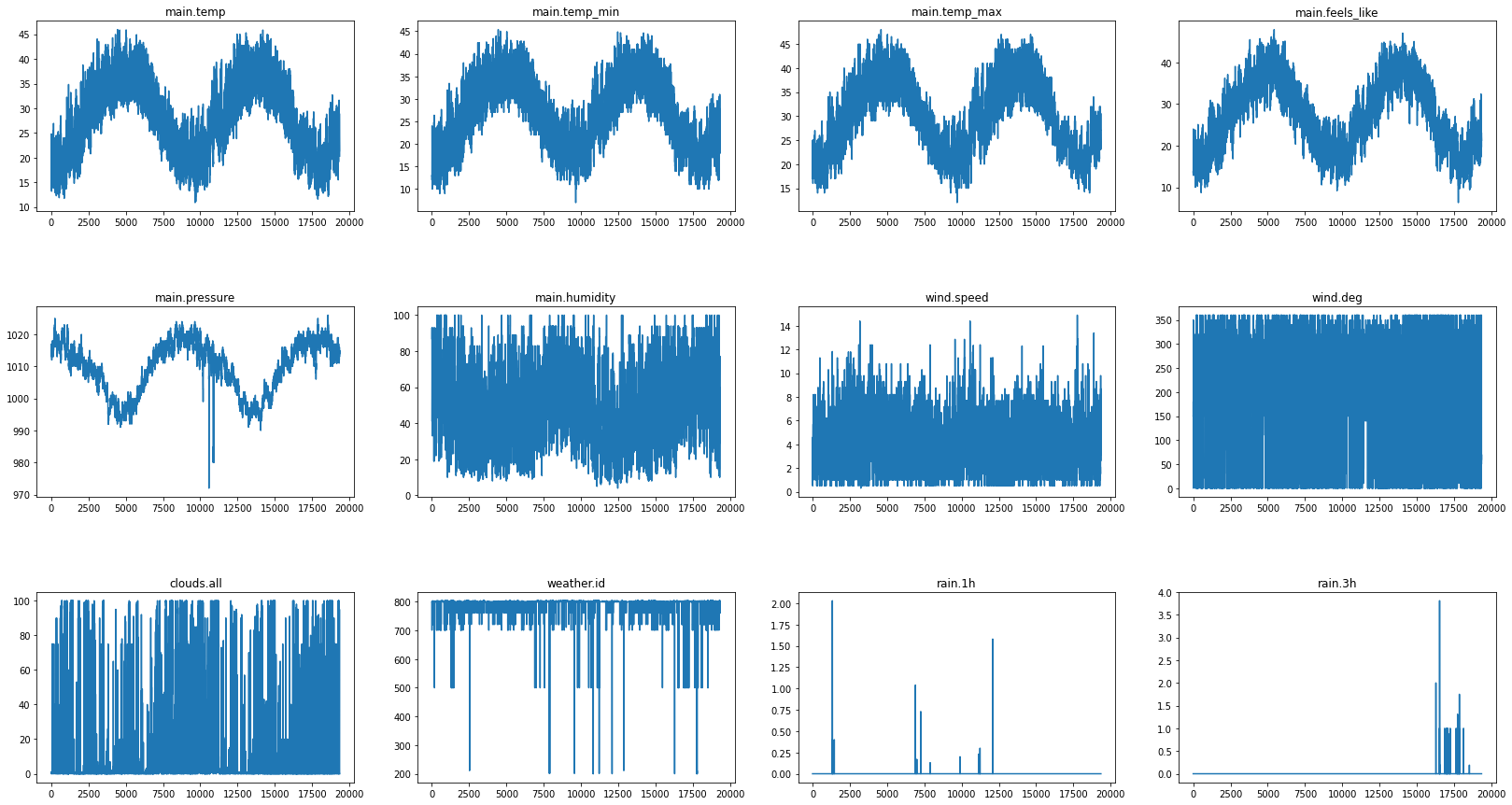
As observed below, temperature and pressure are negatively correlated with each other. Meanwhile, min, max, feels like and average temperature are positively correlated with each other. Therefore, only the temperature should be kept and others can be dropped.
df.sort_values(by=['dt'], inplace=True)
dfwithouttime = df.drop(['dt','dt_iso'], axis=1)
#dfwithouttime=(dfwithouttime-dfwithouttime.min())/(dfwithouttime.max()-dfwithouttime.min()) #normalize
fig, axs = plt.subplots(3, 4, figsize=(28, 15))
fig.subplots_adjust(hspace=.5)
i = 0
j = 0
for col in dfwithouttime.columns:
    dfwithouttime[col].plot(ax=axs[i][j], title=col)
    j += 1
    if j == 4:
      j = 0
i += 1df.drop(['main.temp_min', 'main.temp_max', 'main.feels_like', 'main.pressure'], axis=1, inplace=True)Traffic data
acci_time Accident time
acci_name categorization of the accident
acci_x Latitude
acci_y Longitude
Download data from Dubai Pulse
!wget http://data.bayanat.ae/ar/dataset/ad38cee7-f70e-4764-9c9d-aab760ce1026/resource/025ea6b2-a806-49c2-8294-4f3a97c09090/download/traffic_incidents-1.csv
!wget https://www.dubaipulse.gov.ae/dataset/c9263194-5ee3-4340-b7c0-3269b26acb43/resource/c3ece154-3071-4116-8650-e769d8416d88/download/traffic_incidents.csv
--2020-05-17 11:35:28-- http://data.bayanat.ae/ar/dataset/ad38cee7-f70e-4764-9c9d-aab760ce1026/resource/025ea6b2-a806-49c2-8294-4f3a97c09090/download/traffic_incidents-1.csv
Resolving data.bayanat.ae (data.bayanat.ae)... 185.141.13.100
Connecting to data.bayanat.ae (data.bayanat.ae)|185.141.13.100|:80... connected.
HTTP request sent, awaiting response... 302 Found : Moved Temporarily
Location: https://data.bayanat.ae/ar/dataset/ad38cee7-f70e-4764-9c9d-aab760ce1026/resource/025ea6b2-a806-49c2-8294-4f3a97c09090/download/traffic_incidents-1.csv [following]
--2020-05-17 11:35:30-- https://data.bayanat.ae/ar/dataset/ad38cee7-f70e-4764-9c9d-aab760ce1026/resource/025ea6b2-a806-49c2-8294-4f3a97c09090/download/traffic_incidents-1.csv
Connecting to data.bayanat.ae (data.bayanat.ae)|185.141.13.100|:443... connected.
HTTP request sent, awaiting response... 200 OK
Length: 2716239 (2.6M) [text/csv]
Saving to: ‘traffic_incidents-1.csv’
traffic_incidents-1 100%[===================>] 2.59M 166KB/s in 16s
2020-05-17 11:35:47 (163 KB/s) - ‘traffic_incidents-1.csv’ saved [2716239/2716239]
--2020-05-17 11:35:48-- https://www.dubaipulse.gov.ae/dataset/c9263194-5ee3-4340-b7c0-3269b26acb43/resource/c3ece154-3071-4116-8650-e769d8416d88/download/traffic_incidents.csv
Resolving www.dubaipulse.gov.ae (www.dubaipulse.gov.ae)... 91.73.143.12
Connecting to www.dubaipulse.gov.ae (www.dubaipulse.gov.ae)|91.73.143.12|:443... connected.
HTTP request sent, awaiting response... 200 OK
Length: 6323862 (6.0M) [text/csv]
Saving to: ‘traffic_incidents.csv’
traffic_incidents.c 100%[===================>] 6.03M 170KB/s in 38s
2020-05-17 11:36:29 (163 KB/s) - ‘traffic_incidents.csv’ saved [6323862/6323862]
df1 = pd.read_csv("traffic_incidents.csv")
df2 = pd.read_csv("traffic_incidents-1.csv")
print(df1.dtypes, df2.dtypes)
print(df1.shape[0] + df2.shape[0])
df_union= pd.concat([df1, df2]).drop_duplicates()
print(df_union.shape)
acci_id int64
acci_time object
acci_name object
acci_x float64
acci_y float64
dtype: object acci_id int64
acci_time object
acci_name object
acci_x float64
acci_y float64
dtype: object
79599
(65667, 5)
First of all, only the accident time parameter can be used with weather data, other columns can be drop.
df_union = df_union[['acci_time']]
print(df_union.shape, df_union.acci_time.unique().shape)
df_union.tail
(65667, 1) (64600,)
<bound method NDFrame.tail of acci_time
0 17/05/2020 13:12:42
1 17/05/2020 13:24:43
2 17/05/2020 13:26:02
3 17/05/2020 13:37:07
4 17/05/2020 13:44:31
... ...
23816 27/06/2019 11:21:09
23817 27/06/2019 11:21:35
23818 27/06/2019 11:24:07
23819 27/06/2019 11:24:27
23820 27/06/2019 11:25:26
[65667 rows x 1 columns]>
df_union.acci_time = pd.to_datetime(df_union.acci_time, format='%d/%m/%Y %H:%M:%S')
df_union.sort_values(by=['acci_time'], inplace=True)
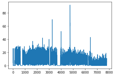
Additionally, the count of the number of traffic accidents occurred within each one hour can be added as one column.
dfh = df_union.groupby([pd.Grouper(key='acci_time',freq='H')]).size().reset_index(name='count')
dfh['count'].plot()
dfh.dataframe tbody tr th {
vertical-align: top;
}
.dataframe thead th {
text-align: right;
}
| acci_time | count | |
|---|---|---|
| 0 | 2019-06-27 10:00:00 | 4 |
| 1 | 2019-06-27 11:00:00 | 19 |
| 2 | 2019-06-27 12:00:00 | 21 |
| 3 | 2019-06-27 13:00:00 | 26 |
| 4 | 2019-06-27 14:00:00 | 0 |
| ... | ... | ... |
| 7800 | 2020-05-17 10:00:00 | 0 |
| 7801 | 2020-05-17 11:00:00 | 0 |
| 7802 | 2020-05-17 12:00:00 | 1 |
| 7803 | 2020-05-17 13:00:00 | 11 |
| 7804 | 2020-05-17 14:00:00 | 5 |
7805 rows × 2 columns
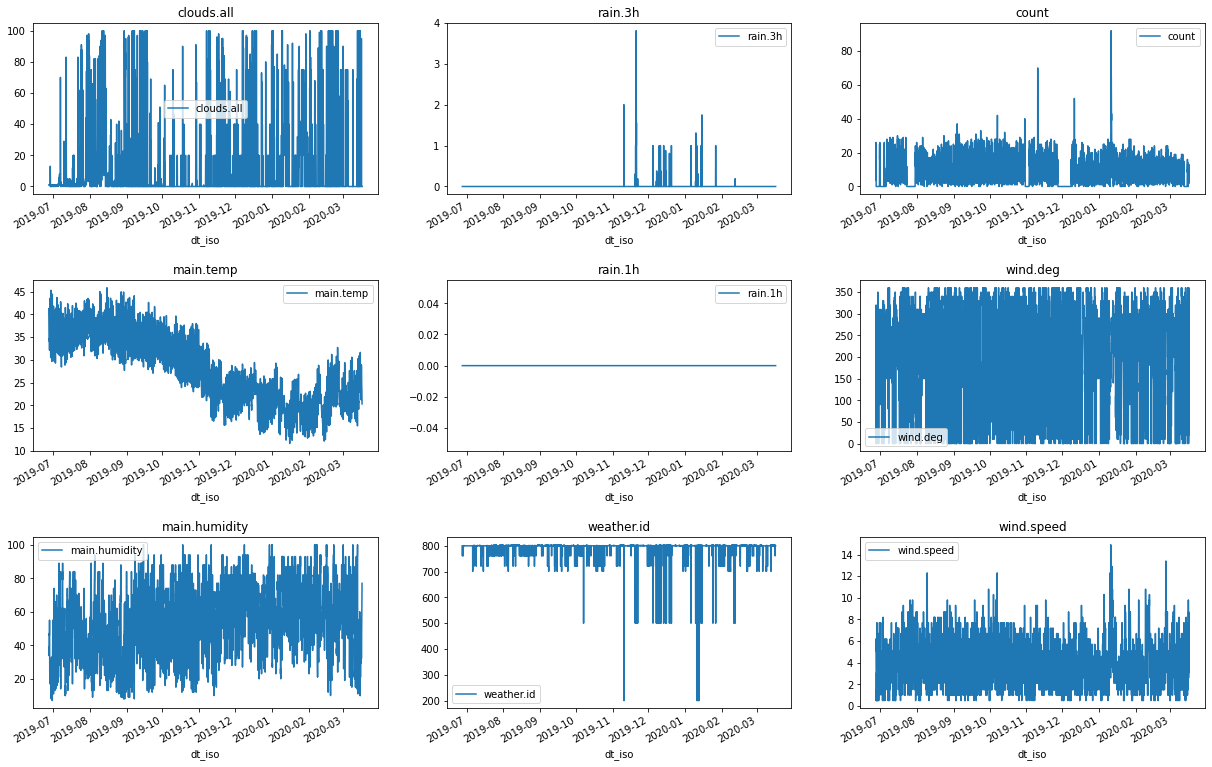
After inner joining weather data and traffic accidents' data, only time range between 2019-06-27 10:00 and 2020-03-16 23:00 with a total of 6327 hours data can be used for analysis.
result = pd.merge(df, dfh, how='inner', left_on=['dt_iso'], right_on=['acci_time'])
result.drop(['acci_time', 'dt'], axis=1, inplace=True)
result.shape
(6327, 10)
fig, axs = plt.subplots(3, 3, figsize=(21, 14))
fig.subplots_adjust(hspace=.5)
i = 0
j = 0
for col in set(result.columns) - set(['dt_iso']):
    result.plot(x='dt_iso',y=col,ax=axs[i][j], title=col)
    j += 1
    if j == 3:
      j = 0
      i += 1
As seen from above, all rain for 1-hour data is 0, so rain 1h can be dropped.
result.drop('rain.1h', axis=1, inplace=True)Interestingly, there are some rain 3-hours cases. After research, there was a flood during that time. Since there is barely raining in Dubai; as a result, drainage measures might not be advanced in Dubai, and there was a significantly increasing number of traffic cases during that time duration.
Important features to predict accident counts per hour
X = result.drop(['count', 'dt_iso'],axis=1)
y = result['count']

X = (X-X.min())/(X.max()-X.min()) # normalize the data
y = (y-y.min())/(y.max()-y.min()) # normalize the data

X_train, X_test, y_train, y_test = train_test_split(X, y, test_size=0.25, random_state=23)
random_forest = RandomForestRegressor(n_estimators=100)
random_forest.fit(X_train, y_train)
rf_feature = pd.Series(random_forest.feature_importances_,index=X.columns)
rf_feature = rf_feature.sort_values()
print(rf_feature[::-1][:5])
fig, axs = plt.subplots(1, 2, figsize=(12, 8))
fig.subplots_adjust(wspace=.5)
rf_feature.plot(kind="barh", ax=axs[0], title='Random Forest')
xgb = XGBRegressor(n_estimators=100)
xgb.fit(X_train, y_train)
xgb_feature = pd.Series(xgb.feature_importances_,index=X.columns)
xgb_feature = xgb_feature.sort_values()
xgb_feature.plot(kind="barh", ax=axs[1], title="XGBoost")
print(xgb_feature[::-1][:5])
main.temp 0.297278
wind.deg 0.255076
main.humidity 0.184519
wind.speed 0.141623
clouds.all 0.074437
dtype: float64
[11:36:35] WARNING: /workspace/src/objective/regression_obj.cu:152: reg:linear is now deprecated in favor of reg:squarederror.
wind.deg 0.430483
wind.speed 0.118081
main.humidity 0.111731
main.temp 0.109670
clouds.all 0.101215
dtype: float32
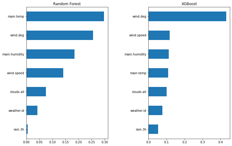
After using both Random forest and XGBoost which are the most popular machine learning algorithms to evaluate the weather and traffic accidents, the windy condition and temperature are important features concluded by both algorithms.
The assumption would be rain is more observable than wind, so people may not go out during the heavy rainy day, and the number of cars decreases. However, people may not be aware of the strong wind, and as a result, the wind has a stronger impact on traffic accidents.
Another assumption would be the temperature also plays an important role in traffic accidents. Perhaps, people should be aware of climate change with greenhouse. Protection of the environment is important to avoid exterme weather condition.
def test(model):
  pred = model.predict(X_test)

def cross_val(model):
  res = cross_val_score(model, X_train, y_train, cv=10, n_jobs=-1)

  print(np.mean(res))

cross_val(xgb)
test(xgb)

cross_val(random_forest)
test(random_forest)
0.21253033333798896
0.21488870400506527
Both models average similar error rates after 10 times cross validation.
Conclusion
The government should make people aware of climate change. Specifically, be aware of wind speed and build cars heavier and more stable.


