A workshop leveraging Azure Machine Learning and introducing its key concepts and mode of operations. A Product overview is available here.
2) For all Azure resources, consider using a prefix that is short and tied to your identity to alleviate the possibilities of name collisions for the azure resources which are URIs.
For instance, consider a 2 or 3 letters prefix withlike: first letter of (first name, middle name, last name).
We'll call this 'prx' as in 'prefix' in the following notes. Note that your prefix should be all lowercase to respect some of the resources naming limitations in Azure.
** Replace 'prx' with your own personal prefix everywhere below **
East US, East US 2, SOuth Central US, West US 2
Create all resources below in the same selection region of your choice. The name of the resource between quotes "(name of resource)" is a good term to use in the search box when creating a resource in the Azure portal.
4) Create a "Resource Group" unless your Azure administrator already created one for you, in that case skip to step #5, but read NOTE (*) below
    Name:       prx-azure-ml-workshop
    Location:   region selected in step #3

Region will not be specified in all instructions below, always set to it to the region you selected in step #3. This is sometimes automatically set if you create a new resource from within your resource group (it will try to default to your resource group's region).

(*) If you have been assigned a resource group already, use it, even if it's not setup in your region of choice (see #3). A resource group is purely virtual and its region has no impact on the resources it contains. In such case, just create the other resources and make sure you specify your region of choice when creating your Azure services.
Everything else left as default (moving forward, when not specified, use the default paramters unless specified in the instructions)
Make sure that all resources below are created within your Resource Group (there will always be an option to change/set the resource group a resource belongs to, make sure it matches yours)
    Workspace Name:     prx-mlws
    Workspace Edition:  Enterprise
6) Get into your Machine Learning workspace instance (created at step #5) and click on 'Launch Now' in the information box in the ML workspace panel.
You can also directly go to https://ml.azure.com/ and select the workspace created in step #5
This will lauch the 'Azure Machine Learning Studio' (referred to as AMLS moving foward) from which all ML resources can be managed and all your ML workflows can be built and executed, deployed from.
    Compute name:           prx-notebook-vm
    Virtual Machine Size:   Standard_D3_v2 or similar (4 vCPUs, 14GB RAM)

    This notebook vm will be used as an editing platform for ml development, it is automatically pre-integrated with the rest of Azure ML.
    Compute name:                   prx-training-cpu
    Virtual Machine Size:           Standard_D3_v2 or similar (4 vCPUs, 14GB RAM)
    Minimal number of nodes:        0
    Maximum number of nodes:        4
    Idle seconds before scale down: 1200 (20 minutes to avoid shutdown/restart times during workshop)
    Compute name:                       prx-training-gpu
    Virtual Machine Size (click 'GPU'): Standard_NC6
    Minimal number of nodes:            0
    Maximum number of nodes:            4
    Idle seconds before scale down:     1200 (20 minutes to avoid shutdown/restart times during workshop)

The two clusters above are 'off' by default (no charge) and are created on-demand when workloads are executed. They autoscale up and all the way down to 0 (complete shutdown) based on the amount of ML workloads thrown at them (multiple ML workloads can be sent to the same clusters). The idle time controls how quickly they may completely shut down.

This enables you to create many different clusters with various configurations (CPU intensive vs Memory intensive vs GPU intensive) and pick the best training cluster for the workload w/o actually paying for anything unless it actually runs (charge is by the minute, from the time a cluster is up, the time it takes to get the cluster up is at no charge).
    Compute name:           prx-inference
    Virtual Machine size:   Standard_D3_v2 or similar (4 vCPUs, 14GB RAM)
    Cluster purpose:        Dev-test
    Number of nodes:        1

    Inference clusters host your ML models deployments. Each deployment (aka ML endpoint) leads to a web service API that will run on an inference cluster. Multiple ML deployed endpoints can co-exist on the same inference clusters, or you can dedicate clusters to specific APIs. The clusters are Kubernetes managed clusters (Azure Kubernetes Service).

    You can also 'attach' existing clusters that your Azure administrators may be managing for you.

NOTE: 'Attached compute' can also be leverage to 'bring your own compute' like a DataBricks cluster or specially tuned VMs of your choice.
Mouse over 'Samples', click on the '...' icon to get the dropdown and select 'Clone' to clone the sample notebooks into your own environment. Select the default target (your own folder already pre-creared) as target and clone the samples into it.
They are 3 Types of experiences to Author ML in Azure ML Studio: Automated ML, Designer, and Notebooks. We will go thru each of them to understand their modes of operations. They all leverage the same underlying Azure ML concepts of Datastores, Datasets, Experimennts, Runs, Compute, etc. but just represent 3 ways to develop Machine Learning models covering the full spectrum from No-Code to Code-Only.
A) Automated ML: trains and finds the best model based on your data without writing a single line of code
We will create an Automated ML experiment to automatically train and find the best model to predict loan approvals based on applicants demographics.
    Web URL:    https://automlsamplenotebookdata.blob.core.windows.net/automl-sample-notebook-data/bankmarketing_train.csv
    Name:       bank-marketing-training
Column headers: All files have same headers
Have a quick look at the data to note that features in the training data set and the 'y' column which we are going to try to predict.
A.4) On the 'Confirm Details' screen, check the 'Profile this dataset after creation' and select your 'prx-training-cpu' compute
Now that we have a dataset, we can click on it, review its content, profile, or potentially update it which will version it.
    Experiment name:            bank-marketing-loan-prediction
    Target column:              y
    Select training cluster:    prx-training-cpu
A.8) On the 'Select task type' screen, select 'Classification' and keep deep learning preview unchecked
Click on 'View additional configuration settings' and observe the parameters available to tune your ML run. No need to change anything. Note the concurrency setting which lets you control how many models run in parallel (one per cluster node max).
Click on 'View featurization settings' to see the controls related to featurization. By default all it automatic, but you could force a specific feature type or imputation model for each feature if needed. Leave all defaults.
A.10) You can monitor the run from the experiment stage. If your cluster is idle, it may take a few minutes for things to kick off. Auto ML also first needs to generate a container image to run the models. The execution will also execute a 'Data guardrails' which will let you know about potential issues in your data for proper training.
We will let this experiment run and get back to it once it's in progress or completed.
Please feel free to check in the first few minutes what's happening, you'll see:
- in the logs the progress of the images being built and misc deployment preparation
- the Data guardrails complete with the results
- the Models being run
You can also go to the 'Compute' section, click on the 'prx-training-cpu' and you'll see the cluster progressively size up to its maximum size as the models get queued up. It should quickly reach its maximum size of 4 nodes as the Auto ML experiment will run about 50 models with this dataset to find the best one for this loan prediction.
As soon as a model completes under this Auto ML experiment, click on it to see its results, including its 'Visualizations' which will help you understand its performance.
Once the AutoML experiment completes, you'll be able to see the best model (auto sorted by Accuracy), look at its Details with Visualizations and its Explanation (auto computed for the best model).
A.11) Click on 'Deploy best model', or go to 'Models' and select the model you wish to deploy if the best selected model is not the one you want to deploy to solve your use case.
    Name:           bank-marketing-loan-prediction
    Compute name:   prx-inference
Click on 'Advanced':
    CPU reserve capacity:       0.1
    Memory reserve capacity:    0.1
Click on 'Deploy' to deploy the model. This will automatically generate a containerized web service deployed in Kubernetes.
Click on 'Endpoints' to monitor the deployment of this endpoint. Once it is completely deployed, you'll be able to access the auto generated Swagger JSON and get access to the 'Consume' endpoint.
B) Designer: enables you to build Azure ML pipelines in a full Drag and Drop environment. This can be used for data preparation to generate training data sets, or end to end to train models.
B.1) Click on 'Designer' in the left menu, and under 'New pipeline', click on the 'Sample 1: Regression - Automobile Price Prediction...' sample to load it up.
B.2) Under 'Settings' which should pop up, select your 'prx-training-cpu' as the Default compute target
Observe the building blocks of this ML pipeline, from source DataSet, to data manipulations, data split, trainig, scoring and evaluation of the model.
To discover the source data set, click on it, then 'Outputs' and then the graphic icon to get a preview of the data with its profiling.
New experiment name: automobile-price-prediction
Click submit to run the experiment pipeline.
You can monitor the progress of the experiment directly from the current screen, you'll see the time icons next to each step conver to green checkmarks as things get executed. Behind the scenes, you just create another ML experiment, which means it's building container images, and starting up the training compute if it was idling.
Therefore, you can also monitor this experiment from the 'Experiments' left side menu item.
Go to 'Designer', load your pipeline from the 'drafts' and click on 'Create inference pipeline'. You have two options here to create two types of endpoints, a real time (one item at a time) endpoint or a batch endoint (batch processing to integrate within an ETL process for instance).
Select 'Real-time inference pipeline'.
The Designer automatically creates a new inference pipeline from the Training pipeline we've been working from, and adds a 'Web Service Input' and a 'Web Service Output' step automatically. This basically transforms our pipeline into a Web Service API. CLick on 'Submit' and then:
Experiment:             Create New
New experiment name:    automobile-price-prediction-realtime
Click 'Submit' and stay on the screen. The pipeline will quickly run to generate the code that will drive this web service.
Once it has completed, click on 'Deploy':
Real-time endpoint name:        automobile-price-rt-endpoint
Compute target:                 prx-inference
Click on deploy.
After a few moments, you'll be able to see your endpoint under 'Endpoints' in the left menu pane. The Swagger URI will be automatically generated as well as the consumption REST API endpoint. It may take a few minutes for the container images to be fully generated and deployed.
B.5) Once the runtime endpoint is in its fully deployed 'Healthy' deployment state, you have the abilty to test it directly from the Portal and get sample integration code for C#, Python and R.
Click on your endpoint, and go to 'Test', then click on Test to execute an API call against the service. Modify the input parameters from here as need to run tests.
Click on your endpoint 'Consume' panel and look at the C#, Python and R integration code snippets.
B.6) Modifying a Designer pipeline does not require a complete rerun. You'll be able to click on the different steps and review their outputs (logs or graphical visualizations) as well as modify them. The pipeline will only need to rerun what's changed and the dependencies, not every step. Its execution context is preserved to speed up iterative work.
Reload your original Designer pipeline and try the following:
- Click on the 'Split Data' step, and modify the split parameter from 0.7 to 0.8. Click on 'Submit' and select the previous experiment to re-execute it. Stay in place to observe the run re-executing only the steps that depend on the change.
- You can monitor and review the output of each step as they complete, without leaving the designer.
We will target a Time Series prediction scenario to introduce some key concepts around working with Azure ML with the Notebook experience.
Concepts to be introduced in this lab session around the Azure ML SDK which enables full access to Azure ML from a Notebook experience:
- Workspace integration: how to connect your notebook to your AML Workspace to leverage all its resources
- Targetting AML Compute resources
- Creating Compute Configuration to properly manage your code libraries dependencies and enforce tight control of the runtime computes
- Data access via DataSets (see examples above), DataReferences (ability to reference data directly in the Data Lake), and PipelineData (enabling exchange of intermadiate data between pipeline steps)
- Pipeline Steps: input/output/dependency control, re-usability to leverage 'compute only when needed'
- Building a pipeline and running it via an Azure ML Experiment
- Full Monitoring of execution from Notebooks
- Access to intermediate data steps for debugging
We'll go thru the following:
- Quick Review of a Time Series example via AutoML in the portal with a sample data use case
- Use of real life disparate data sources to build an engineering pipeline to generate a training data sets for a time series scenario
- Leverage of this data set in an AutoML Experiment (via UI or via Notebook step)
Go to https://ml.azure.com and click on Automated ML, then 'New Automated ML run'
Follow the instructions from this example: https://docs.microsoft.com/en-us/azure/machine-learning/tutorial-automated-ml-forecast
PLEASE MAKE SURE to ignore the two columns 'casual' and 'registered' from the dataset as they are breakdown values of the 'cnt' column we're trying to predict.
NOTE: leverage the existing CPU compute created in the previous parts of this workshop. No need to create a new one.
We will kick off the experiment, and get back to the results later. This should take from 10 to 20 minutes depending on your cluster configuration.
Use Case #1: time series predictions
Input Datasets:
- h_time_series_1: hourly time series with multiple features that need to be pivoted. Date + Hour columns.
- h_time_series_2: hourly time series with multiple features that need to be pivoted. Date + Hour columns.
- h_time_series_3: hourly time series, no need to pivot. Date + Hour columns.
- d_time_series_1: daily time series with one feature, date column needs reformatting
- d_time_series_2: daily time series containing the column to predict, date column needs reformatting

We will build a data engineering pipeline which prepares a training data sets combining all these data sources:
- Steps: pivot h_time_series_1, h_time_series_2, h_time_series_3 -> P1,P2,P3
- Step: join the 3 pivotes series -> P1 U P2 U P3 -> H
- Step: aggregate the joined data at a day level, and generate statistical values for each day (24 hourly data points summarized as min, max, mean, etc.) -> H -> H_D
- Step: join two hourly series, and clean up dates -> D
- Step: join H_D with D -> H_D U D to generate the infal data set -> F
Here is an output of the final pipeline we will build to accomplish the data preparation for this use case:
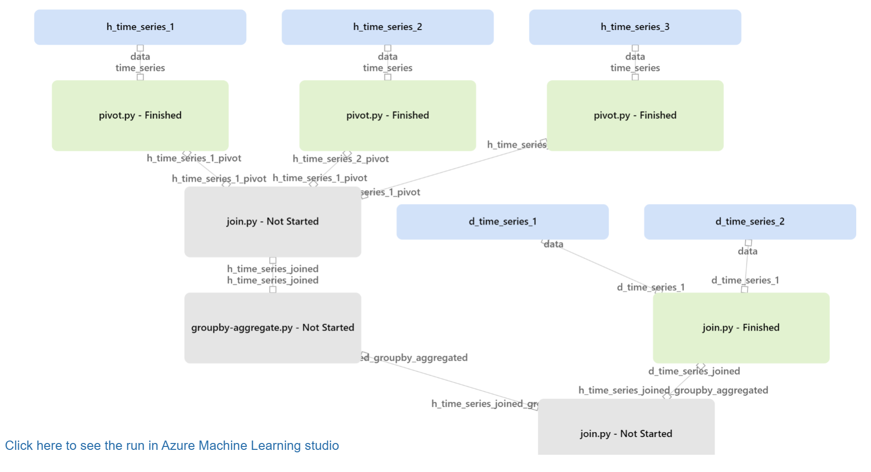
A notebook is available that constructs all these pipeline elements: https://github.com/aldelar/azure-machine-learning-workshop/use-case-1/use-case-1/data-prep-pipeline.ipynb
The notebook final step geneates a DataSet named 'use-case-1-d' for the daily level combined features. This is the data set to leverage to run AutoML for time series as done in C. Consider using Deep Learning with a GPU cluster.
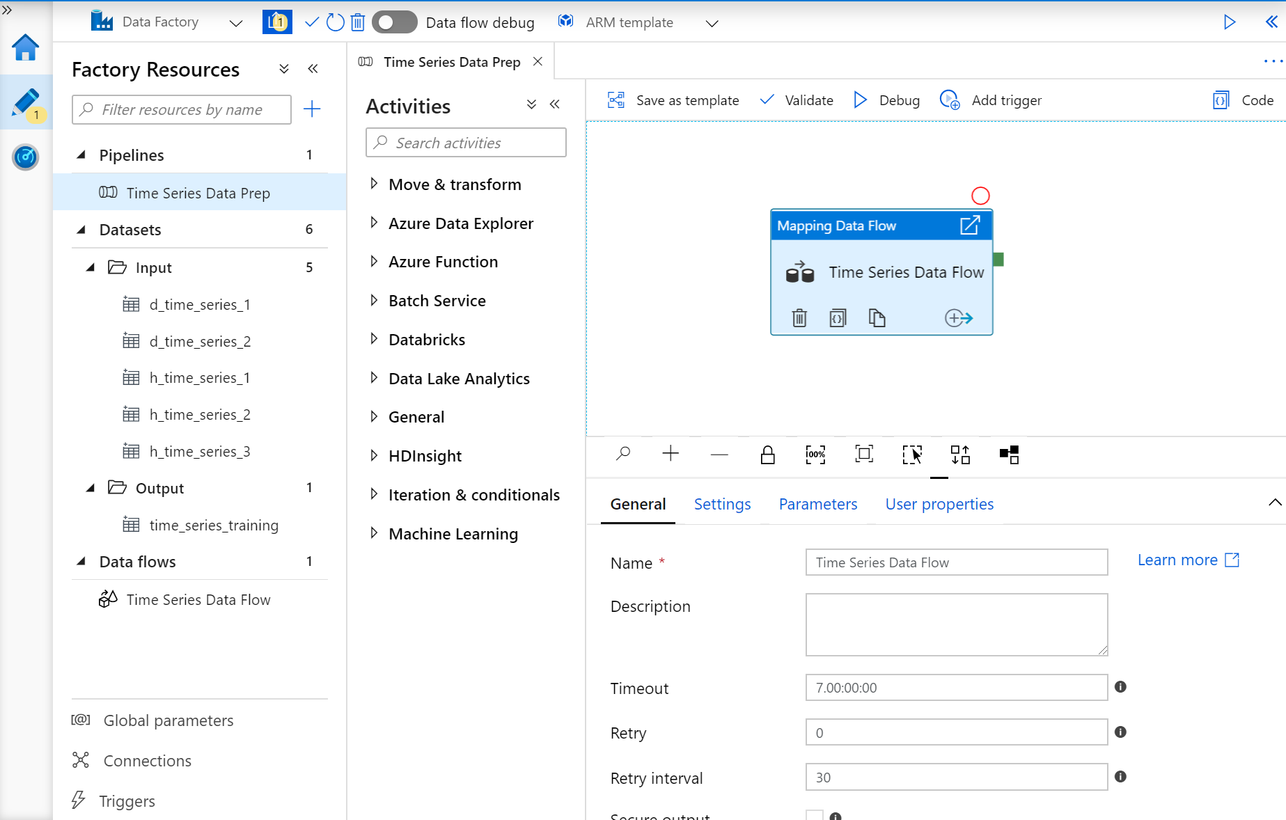
We will create a simple Pipeline which leverages one DataFlow, connected to 5 input Datasets, generating one output Dataset. Here's the output of what we're building below:
Let's build all these elements before we get into the Data Flow.
    Name:       prx-adf
    Version:    V2
    Git:        Unchecked for this quick workshop, but recommended otherwise
Once created, you can jump to the Data Factory studio via https://adf.azure.com/
Click on 'Connections' at the bottom left of the screen Create a '+ New' connection Select 'Azure Blob Storage' (this is the storage type that comes default with AML, we'll connect to it to source the files you uploaded in the sections above)
Name: prx_data_lake
Pick your subscription from the subscription dropdown, then pick the 'Storage account name' from the list below that starts with 'prxmlws#########' where ######## is a series of digits auto created by AML. 'prx' is your unique prefix defined early on.
Click 'Test Connection' to make sure it works, and then 'Create'
Click on '...' next to Datasets on the left menu pane, and select 'New Dataset'. Select 'Azure Blob Storage' from the source storage option pane (you can search for it), click 'Continue' and select 'DelimitedText' as the format.
Name:                   h_time_series_1
Linked service:         aml_data_lake
First row as header:    checked
Then browse to find your file that represents the first hourly time series (aka 'time series 1'). Click OK to create the dataset.
Once created, it should show up on a new tab, click on the 'Connection' subtab, and then 'Preview Data' to make sure you configured it correctly.
NOTE: Click on 'Validate all' to make sure there's no error and then 'Publish all' to save the new objects.
E.4) Repeat E.3 for the following datasets: h_time_series_2, h_time_series_3, d_time_series_1, d_time_series_2
The easiest way to do this is to leverage the 'Clone' feature.
Click on the '...' next to your dataset name in the left pane menu, and click 'Clone'.
Once cloned (it should appear in a new tab), update it's name to be 'h_time_series_2', then click on 'Connection' and 'Browse' to select the file that represents the second hourly time series. Once selected, click on 'Schema' and 'Import Schema', select 'From Connection/Store' to bring in the new columns.
Check that everything is ok with 'Preview Data'.
Repeat the cloning process 3 times to create h_time_series_3, d_time_series_1, and d_time_series_2
Rename it 'Time Series Data Prep' Open up the 'Move & transform' section and drag and drop a 'Data flow' activity. Select 'create new dataflow' and then select 'Mapping DataFlow'
A new DataFlow canvas opens up. Rename it to 'Time Series Data Flow'
Click on 'Data flow debug' on the top menu bar to kick off the debug runtime (it takes a few minutes).
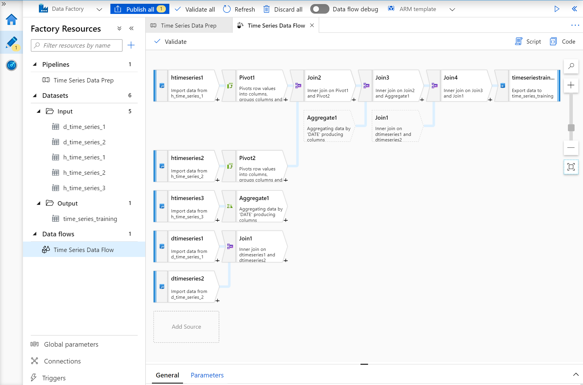
Here's the full output of the Data Flow we are about to build as reference. Some of the steps are using the default generated names and you should end up with the same names if you follow the instructions in the same order.
Add 3 Data Sources by clicking the 'Add Source' box in the canvas, and select 'h_time_series_1' from the drop down. Rename it as well propely like 'htimeseries1' (note: no space or _ allowed for the names). Repeat the process for 'h_time_series_2' and 'h_time_series_3' datasets to set them as data sources for the Data Flow.
'htimeseries1': Click on '+' nexy to the first source and select 'Pivot' Select 'MYDATE' for the 'Group By' parameter Select 'NODE_ID' for the Pivot Key Go to 'Pivoted Columns' and click in "Pivot Expression" and type 'min(MW)' in the editor in the righ pane that pops up. This pane allows you to build very complex transformations as needed. We'll just use it now to create some basic statistical aggregates from the hourly data by aggregating at the date level. Click "Save and Finish", and then name this 'min_' in the box next to the expression we just entered to prefix the column name with 'min_'. Click on '+' to add a second aggregate expression: set it to 'max(MW)' and name the prefix 'max_'
Click on 'Data Preview' and validate that you get a pivoted table with 4 columns, min/max aggregates by day for each NODE_ID type, you should get MYDATE,min_N1,min_S1,min_Z1,max_N1,max_S1,max_Z1 as columns.
'htimeseries2': Repeat the pivot operations above for the 'htimeseries2' source. This time you should end up with 5 columns as NODE_ID has only two distinct values.
'htimeseries3': Add an 'Aggregate' step for this time series as there's no column to pivot. Group by 'DATE' Aggregates:
- type in min_CLOAD in the first drop down to create a new column
- type in min(CLOAD) in the expression box next to it to define the aggregate
- click on '+' and select 'add column' to add a new column
- type in max_CLOAD in the first drop down to create a new column
- type in max(CLOAD) in the expression box next to it to define the aggregate Click on 'Preview Data' to validate the aggregation for this input.
'dtimeseries1' and 'dtimeseries2':
- add them as new sources by selecting the corresponding datasets and renaming them properly
- click on '+' next to 'dtimeseries1' and add a 'join' Select the 'Right stream' to be 'dtimeseries2' Under Join conditions, select RDATE on both sides. Click 'Preview data' to validate that the join works properly.
Repeat the operation:
- Join 'Pivot1' with 'Pivot2' on 'MYDATE'
- Join 'Join2' and 'Aggregate1' on 'Pivot1@MYDATE' and 'DATE'
- Join 'Join3' and 'Join1' on 'Pivot1@MYDATE' and 'dtimeseries1@RDATE' Click on 'Data Preview' for 'Join4' which should bring all these data sets together
Now, let's clean up the output by removing columns and renaming them.
Add a 'sink' at the end of 'Join4' to store the final dataset:
- name it 'timeseriestraining'
- sink dataset: click on 'New', select 'Azure Blob Storage', then 'DelimitedText', name it 'time_series_training' and select 'aml_data_lake' in the service dropdown and browse to your 'datasets' folder, select it. Then add '/time-series-training' in the second box of the path to automatically create a folder as it doesn't exist yet.
- check 'first row as header'
- set import schema to 'None'
- click 'Create'
Now click on 'Validate all', and then 'Publish all'.
Go back to the pipeline, and click 'Debug' to run everything and generate the training file. While it's running, you can click on the 'glasses' icon and see the details of the run, step by step with statistics about each step.
Go to https://ml.azure.com to get back into your Azure ML Workspace. Create a new DataSet 'from datastore':
            Name:           d_use_case_1_adf
            Type:           Tabular
            Datastore:      workspaceblobstore
When asked to 'Browse', select your 'datasets' folder, and then select the 'time-series-training' folder. DO NOT select the file, so that the dataset can work independently of how the data is generated into this folder (either a single file or multiple files).
Click on 'Next' and make sure you delect 'Column headers' to be 'all files have same headers'.
Click 'Next' and MAKE SURE YOU UNSELECT THE DUPLICATE TIME COLUMNS to only keep 'DATE' for instance (in that case unselect RDATE and MYDATE).
Click on 'Next' and select 'Profile this dataset after creation' against your CPU compute.
E.8) Use your Data Factory generated DataSet as a training set for an AutoML Experiment to predict X2 from the available features
Click on Automated ML on the left menu pane and create a new AutoML Experiment.
Select the 'd_use_case_1_adf' dataset you just created.
Call the experiment 'd_use_case_1_adf_automl', and select 'X2' as the target column.
On the next screen select 'Time series forecasting' as a task type, and select 'DATE' as the time column.
Click 'Finish' to kick off the Experiment.
Feel free to create a second AutoML run against the same dataset but with 'Deep Learning' enabled. You can, and probably SHOULD to keep things together, reuse the same experiment when you create the second run using Deep Learning. You are afterall trying to solve the same problem but just with a different approach. If you have two training clusters, you could send each job against a different cluster to parallelize this accordingly. If sent to the same clusters, the jobs of each experiment will compete for compute and stagger as they come.
This concludes this chapter around Use Case 1 to take care of data prep in a full code environment with Notebooks and Azure ML Pipelines, or in a full No Code environment with Azure Data Factory and Azure DataFlow.
Use Case #2: time series clustering
In this use case, we're trying to see how to easily cluster about 700 time series of hourly data over a period of 45 months.
We will leverage Azure Data Explorer (aka ADX), which is a fast, fully managed data analytics service for real-time analysis on large volumes of data streaming from applications, websites, IoT devices, and more.
Search for 'Data Explorer' in your Azure Portal 'new resource' panel, and use the following settings (reminder: prx is your own 'prefix'):
            cluster name:           prxadx
            region:                 same region than your other resources
            resource group:         same as previously used
            compute specifications: Dev(No SLA)
Keep all other settings as default and click 'Create'.
Once the service is created, click on it in your resource group and click on the 'configuration' item in the left pane, select Python and R and 'Save':
Click on '+ Create Database' in your Azure ADX cluster resource.
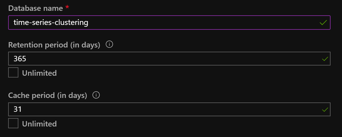
Set the parameters the following way:
The retention period indicates when data that gets loaded today will be automatically deleted (here set to one year from today), and the cache period indicates which part of the data is cached in the local nodes (on SSD disk and/or memory). You can choose to have the entire data set cached if needed, as long as your nodes have enough SSD cache. They are a lot of node types that can accomodate different scenarios.
Click on 'Overview' in your ADX resource, and copy the URI.
Paste the URI into a new browser window, it should look like this:
https://your_adx_cluster_name.your_region.kusto.windows.net
You also have the option to work from a Desktop Client, which can be downlaoded here:
The rest of this workshop assumes working from the Web UI client.
Click on 'Add Cluster' and type 'help' in the URI box (only put 'help', nothing else, it's a handy shortcut that gets interpreted), then click 'Add', and you will have a new cluster attached to your configuration with some sample datasets.
These datasets are used in some of the documentation examples to be found here:
Azure Data Explorer Documentation
Download this .kql (Kusto Query Language, Kusto being the code name for ADX) file: time-series-clustering.kql
Now in the Studio Web UI, on the top right side, click on the 'File' menu icon and 'Open' to select this file and open it in the Studio.
If you do not see your cluster already registereed on the left side panel, click on 'Add Cluster' and enter the full URI of your cluster (See section F.4 to find the URI).
Make sure you click on the database created in step F.3 which should be under your cluster to set the 'context' of the .kql file you just loaded into the Web UI client.
At this point you are getting ready to follow the script and its instructions.
Here are the preparation steps needed to load data from an Azure Data Lake.
Assuming we're re-using the blob storage account that was created at the beginning of this workshop, navigate to it and upload all the .csv. files which are present under this folder:
Download them locally, then upload them into a container in your blob storage account.
We'll then need to obtain SAS token to replace the different parts of the script which are currently set to things like:
_blob_SharedAccessSignature_URI_for_congestion_file_1 _blob_SharedAccessSignature_URI_for_congestion_file_2 ... _blob_SharedAccessSignature_URI_for_geo_file
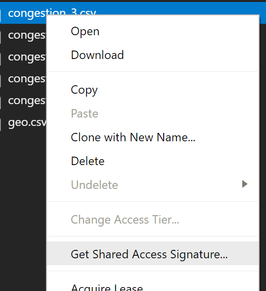
We'll need to obtain a SAS URI for each of these files. Do do this, once uploaded, the easiest is to use Azure Storage Explorer, login to your Azure account, then navigate to your blob storage account and container with all these files.
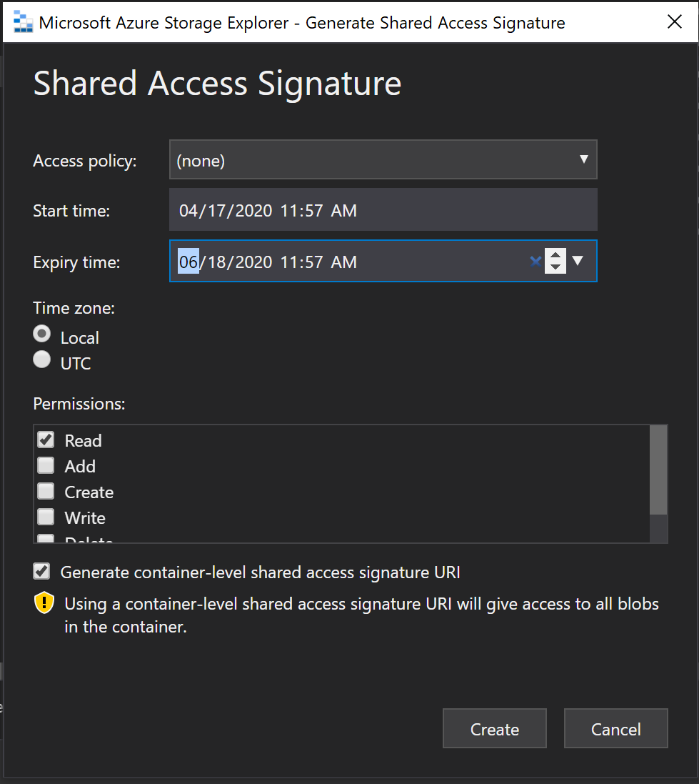
Then right click on one of the files to generate a SAS token:
On the next screen, make sure you select 'generate container level shared access signature URI' to get a token that will work for all files in this container. You can keep the rest of the defaults which enables only ready/list on the container, and change the expiration date accordingly (a week, etc. depending on how long you want the token to be valid).
The token you will get will be a full URI with access keys in it. It's on the next screen in the 'URI' box, copy that.
You will be able to update the File Name which is included somewhere in the middle of it, to point to any file name in this container.
Go to the .kql scrip, and replace the URI items with the URI you got, and then update the file it references to be the correct file in each location.
You will see that the 'congestion' data has been split into 7 files, copy the URI 7 times, then replace the file name in the middle of it to point to each file.
Do the same thing for the 'geo' file, replacing the file name in the middle of the URI with 'geo.csv'.
At this point you should be ready to go over each step of the .kql file and proceed with the execution.
Example of URI:
https://some_blob_ref.blob.core.windows.net/azureml-blobstore-xyzxyzxyz/datasets/time-series-clustering/congestion_1.csv?(some-params-representing-the-key-do-not-change)
Copy this URI everywhere there needs to be one, and replace 'congestion_1.csv' with the different file names as needed.
Since we generated a container level SAS, the same URI pattern can be applied to any file in this container instead of generating a SAS token for each file individually.
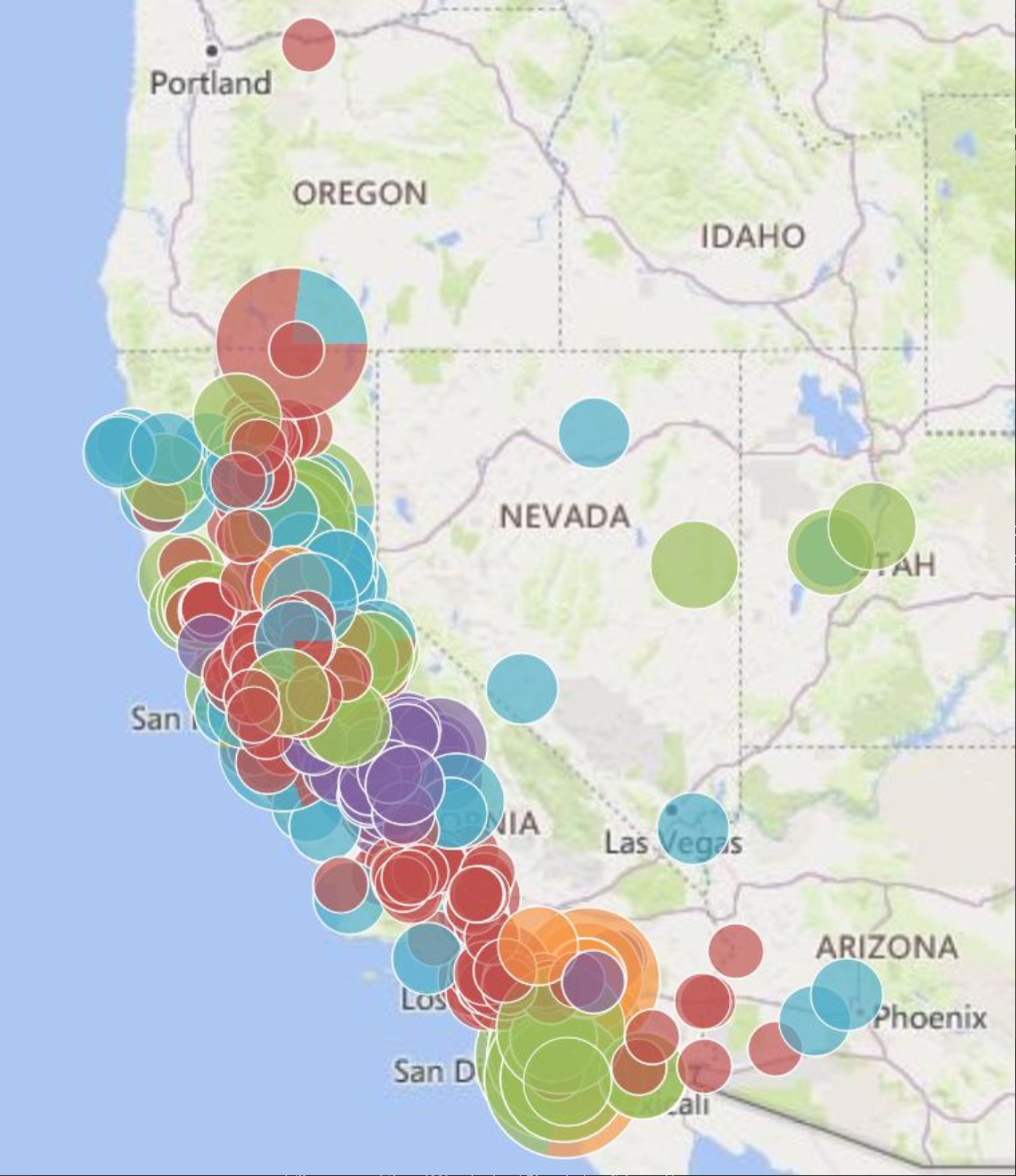
At the end of the script, you should be able to visualize clusters on a map based on a k-means clustering from features generated via ADX:
- basic statistical information
- auto detected signal periods
autocluster() is also used as another built-in approach to cluster time series.
Azure ML comes with a data engineering specific set of libraries called 'dataprep'. This SDK package enables to build Azure ML SDK Dataprep 'Data Flows' which can be piped with each other and support data clustering for large scale transformations.
Getting Started Python Notebook
A lot of common data prep scenarios covered in dedicated Jupyter Notebooks
This notebook covers in details a full data prep implementation of 'Use Case 1' using only the Azure ML SDK Dataprep. It builds a simple one step pipeline which executes a series of Dataprep DataFlow transformations.
Have a look at this Notebook and execute it in your Azure ML environment: azureml-dataprep-sdk.ipynb
We will leverage the DataFlow built in section E) to expand it with a few steps to implement a few extra common data engineering scenarios.
Scenarios:
- lag features
- categorization
- one hot encoding
- replacing missing values with defaults
We will edit the original Data Flow to generate this updated version:
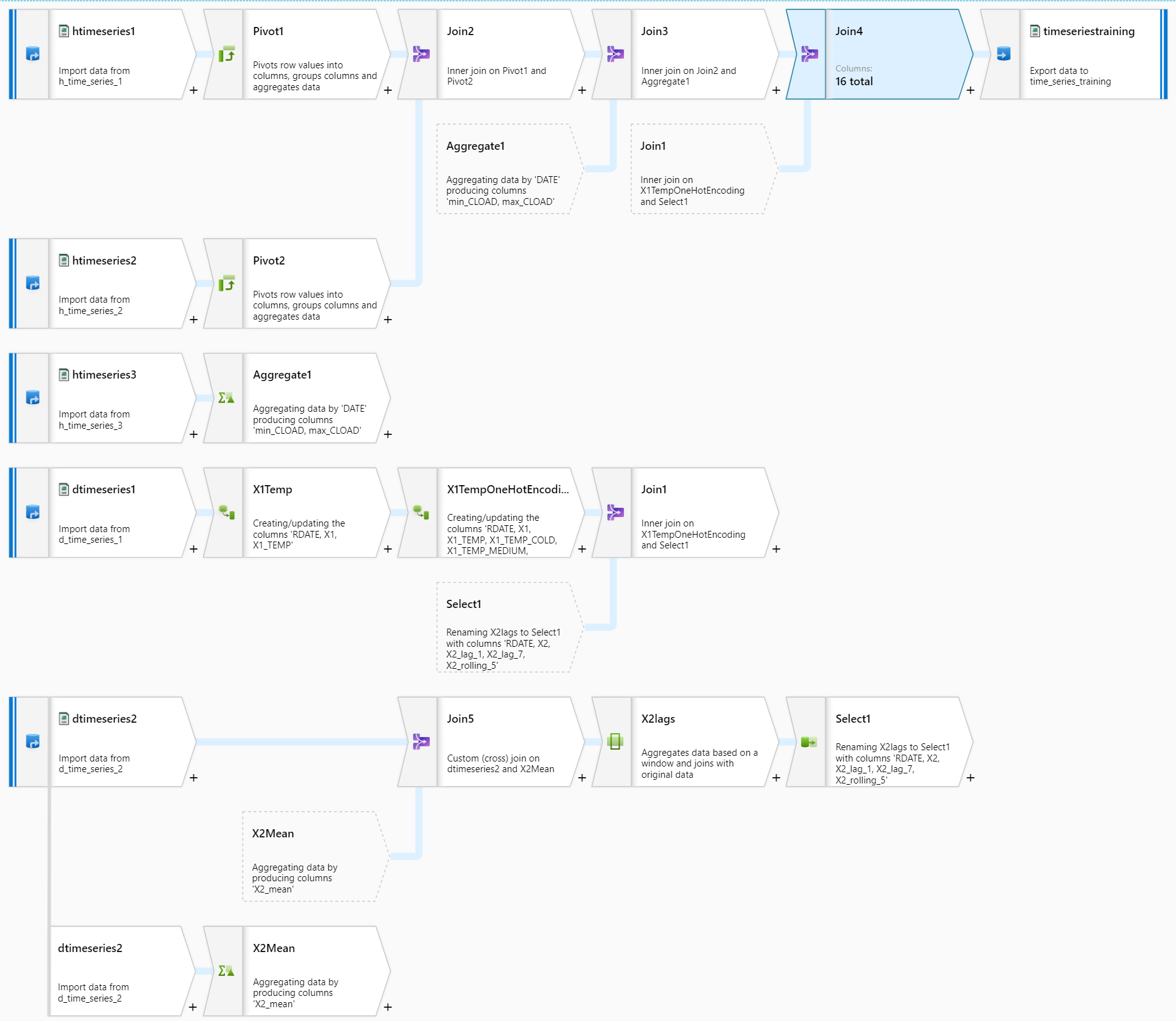
Edit the Dataflow as found in E.6) and add the following steps:
-
Add a step right after 'dtimeseries1' of type 'Derived column' and name it 'X1Temp'. We will generate the 'TEMP' categorization feature column
X1_TEMP iif(X1 < 60, 'COLD', iif(X1 > 80, 'HOT', 'MEDIUM')) -
Add a new 'Derived column' step right after 'X1Temp' and name it 'X1TempOneHotEncoding' where we will implement 3 columns to take care of the encoding:
X1_TEMP_COLD iif(equals(X1_TEMP, 'COLD'),1,0) X1_TEMP_MEDIUM iif(equals(X1_TEMP, 'MEDIUM'),1,0) X1_TEMP_HOT iif(equals(X1_TEMP, 'HOT'),1,0) -
Add an 'Aggregate' step after 'dtimeseries2', call it 'X2Mean', to generate a new X2_mean column (no group by column), effectively just computing the mean value of X2 once for re-use in subsequent steps where needed to 'fill in' missing values
Group by: none Aggregates: X2_mean mean(X2) -
Add 'Join5' at the end of 'dtimeseries2' and join it to the new 'X2Mean'
Right Stream: X2Mean Join type: Custom (cross) Condition: true() -
Add a 'Window' schema modifier step after 'Join5' and call it 'X2lags'. We will create 3 lagging features (lag of 1 period, lag of 7 periods, and a rolling average of past 5 periods). We will also setup a default value of 'X2_mean' for each missing value in the new lags columns
1.Over (left blank) 2.Sort RDATE Ascending 3.Range by Unbounded 4.Window columns X2_lag_1 iifNull(lag(X2,1),X2_mean) X2_lag_7 iifNull(lag(X2,7),X2_mean) X2_rolling_5 iifNull((lag(X2,1)+lag(X2,2)+lag(X2,3)+lag(X2,4)+lag(X2,5))/5,X2_mean) -
Add a 'Select' step after the 'X2lags' step to remove the X2_mean column from the dataset
Keep all defaults and simply click on the 'delete' icon next to the X2_mean row in the mapping definition to remove that column from the dataset.
- Update 'Join1' to join from 'Select1' instead of the previously set 'dtimeseries2' stream
