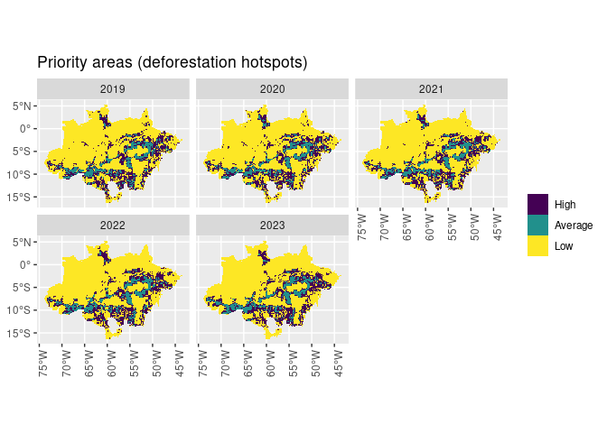
This package introduces a method for prioritizing deforestation hotspots to support law enforcement actions in the Brazilian Amazon, as describen in the paper entitled: Science-based planning can support law enforcement actions to curb deforestation in the Brazilian Amazon by Mataveli et at. (2022) [1], available at https://doi.org/10.1111/conl.12908
This is the abstract of the aforementioned paper [1]:
While Brazil publicly committed to reduce deforestation in Amazonia at the 26th Conference of the Parties (COP26), the Brazilian parliament is moving toward weakening environmental laws. Deforestation rates continue ascending, reaching in 2021 the highest value since 2006 (13,235 km2). To overcome this paradox, strategies to curb deforestation are mandatory. The current strategy, “Plano Amazônia 21/22,” prioritizes law enforcement actions to curb illegal deforestation in only 11 Amazonian municipalities. Here, we show that this prioritization is likely to be insufficient since these municipalities account for just 37% of the current deforestation rate. This strategy may also be undermined by the leakage of deforestation actions to unmonitored municipalities. Using a set of spatially explicit datasets integrated into a deforestation-prediction modeling approach, we propose a science-based alternative method for ranking deforestation hotspots to be prioritized by law enforcement actions. Our prioritization method accounts for more than 60% of the deforestation, detecting larger deforested areas in both private and public lands, while covering 27% less territory than “Plano Amazônia 21/22.” Optimizing the detection of priority areas for curbing deforestation, as proposed here, is the first step to reducing deforestation rates and comply with the Brazilian legal commitment of 3925 km2 year−1.
[1] Mataveli, G., de Oliveira, G., Chaves, M. E., Dalagnol, R., Wagner, F. H., Ipia, A. H., … & Aragão, L. E. (2022). Science‐based planning can support law enforcement actions to curb deforestation in the Brazilian Amazon. Conservation Letters, e12908.
You can install the latest version of prioritizedeforestationhotspots from GitHub:
# install.packages("devtools")
devtools::install_github("albhasan/prioritizedeforestationhotspots")This basic example produces results similar to those shown in the aforementioned paper (note that estimating the model accuracy takes hours!):
library(sf)
library(prioritizedeforestationhotspots)

# Run the model
out_dir <- "~/Documents/prioritize_res"
# NOTE: This takes long to run!
estimate_accuracy(out_dir)
fit_model(out_dir)
results_to_shp(out_dir)If you don’t have time to run the model, you can just load the results already stored in the package. This example shows the deforestation hotspots in a map:
library(prioritizedeforestationhotspots)
library(dplyr)
library(ggplot2)
library(purrr)
library(sf)
library(tidyr)
library(tidyselect)
library(tools)

# Read the result data from the package.
priority_sf <-
    system.file("extdata", "results", "priority_classes.shp",
                package = "prioritizedeforestationhotspots") %>%
    read_sf()

# Format the data.
priority_tb <-
    priority_sf %>%
    st_drop_geometry() %>%
    pivot_longer(cols = starts_with("pri"),
                 names_prefix = "pri",
                 names_to = "ref_year",
                 values_to = "priority")

# Arrange data into a sf object.
priority_sf <-
    priority_sf %>%
    select(id) %>%
    right_join(priority_tb,
               by = "id",
               multiple = "all") %>%
    mutate(priority = factor(priority,
                             labels = c("High", "Average", "Low"),
                             ordered = TRUE))

# Plot.
priority_sf %>%
    ggplot() +
    geom_sf(aes(fill = priority), lwd = 0) +
    facet_wrap(~ref_year) +
    theme(axis.text.x = element_text(angle = 90)) +
    theme(legend.title=element_blank()) +
    ggtitle("Priority areas (deforestation hotspots)")
We also included the variables used for the model. This example shows some of the data included in this package:
library(prioritizedeforestationhotspots)
library(dplyr)
library(tidyr)
library(sf)
library(ggplot2)

def_sf <-
    deforestation_grid %>%
    right_join(deforestation_data, by = "id")

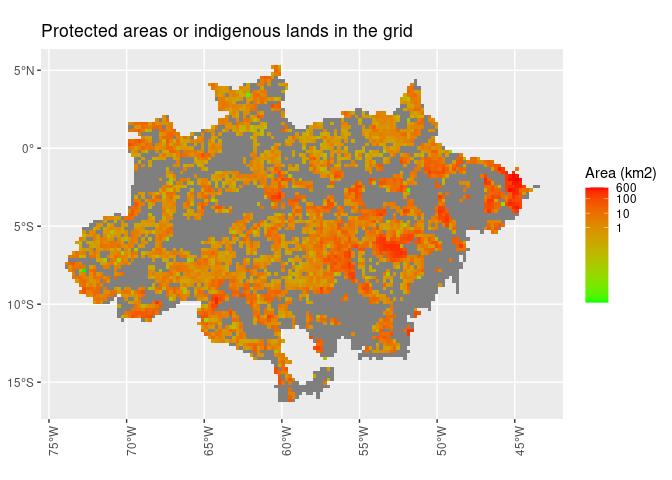
def_sf %>%
    ggplot() +
    geom_sf(aes(fill = area_PA), lwd = 0) +
    scale_fill_gradient(name = "Area (km2)",
                        trans = "log",
                        breaks = c(1, 10, 100, 600),
                        low = "green",
                        high = "red") +
    theme(axis.text.x = element_text(angle = 90)) +
    ggtitle("Protected areas or indigenous lands in the grid")
#> Warning: Transformation introduced infinite values in discrete y-axis
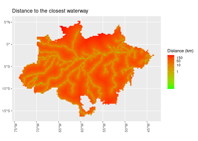
def_sf %>%
ggplot() +
geom_sf(aes(fill = dist_hidro), lwd = 0) +
scale_fill_gradient(name = "Distance (km)",
trans = "log",
breaks = c(1, 10, 50, 150),
low = "green",
high = "red") +
theme(axis.text.x = element_text(angle = 90)) +
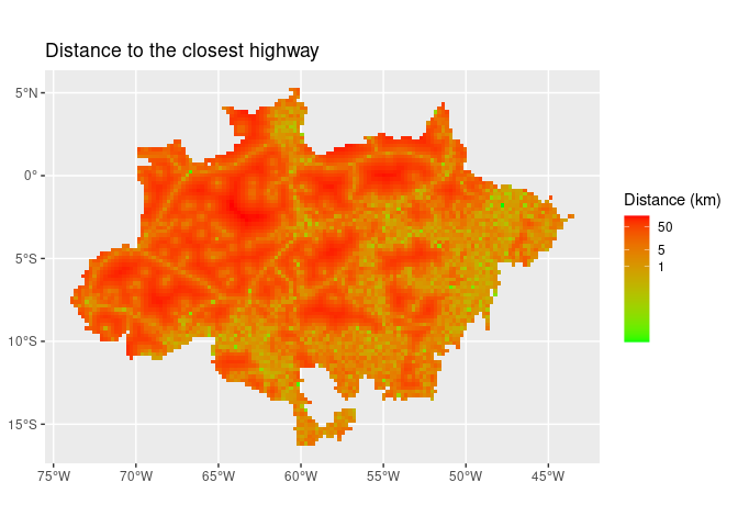
ggtitle("Distance to the closest waterway")def_sf %>%
ggplot() +
geom_sf(aes(fill = dist_road), lwd = 0) +
scale_fill_gradient(name = "Distance (km)",
trans = "log",
breaks = c(1, 5, 50),
low = "green",
high = "red") +
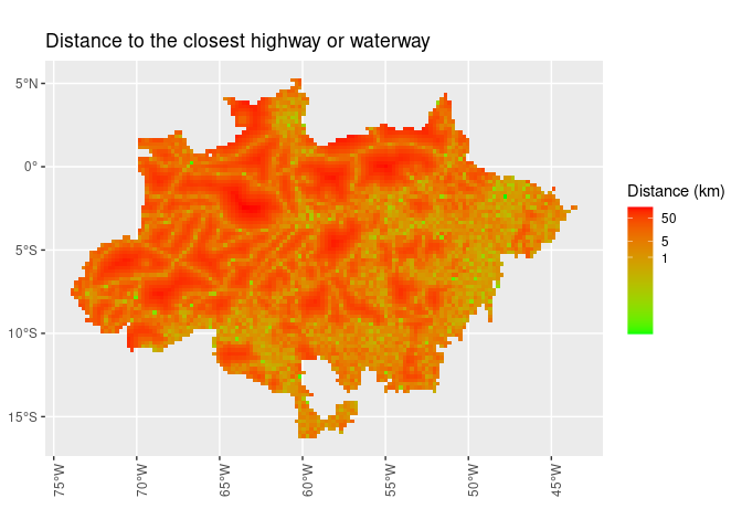
ggtitle("Distance to the closest highway")def_sf %>%
ggplot() +
geom_sf(aes(fill = dist_road_hidro), lwd = 0) +
scale_fill_gradient(name = "Distance (km)",
trans = "log",
breaks = c(1, 5, 50),
low = "green",
high = "red") +
theme(axis.text.x = element_text(angle = 90)) +
ggtitle("Distance to the closest highway or waterway")def_sf %>%
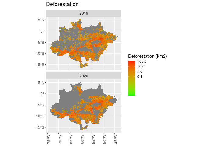
drop_na(def) %>%
ggplot() +
geom_sf(aes(fill = def), lwd = 0) +
scale_fill_gradient(name = "Deforestation (km2)",
trans = "log",
breaks = c(0.1, 1, 10, 100),
low = "green",
high = "red") +
facet_wrap(~ref_year, ncol = 1) +
theme(axis.text.x = element_text(angle = 90)) +
ggtitle("Deforestation")
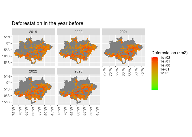
#> Warning: Transformation introduced infinite values in discrete y-axisdef_sf %>%
ggplot() +
geom_sf(aes(fill = def_1_ly), lwd = 0) +
scale_fill_gradient(name = "Deforestation (km2)",
trans = "log",
breaks = c(0.01, 0.10, 1, 10, 100),
low = "green",
high = "red") +
facet_wrap(~ref_year) +
theme(axis.text.x = element_text(angle = 90)) +
ggtitle("Deforestation in the year before")
#> Warning: Transformation introduced infinite values in discrete y-axisdef_sf %>%
ggplot() +
geom_sf(aes(fill = def_2_ly), lwd = 0) +
scale_fill_gradient(name = "Deforestation (km2)",
trans = "log",
breaks = c(0.01, 0.10, 1, 10, 100),
low = "green",
high = "red") +
facet_wrap(~ref_year) +
theme(axis.text.x = element_text(angle = 90)) +
ggtitle("Deforestation 2 years before")
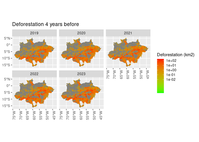
#> Warning: Transformation introduced infinite values in discrete y-axisdef_sf %>%
ggplot() +
geom_sf(aes(fill = def_4_ly), lwd = 0) +
scale_fill_gradient(name = "Deforestation (km2)",
trans = "log",
breaks = c(0.01, 0.10, 1, 10, 100),
low = "green",
high = "red") +
facet_wrap(~ref_year) +
theme(axis.text.x = element_text(angle = 90)) +
ggtitle("Deforestation 4 years before")
#> Warning: Transformation introduced infinite values in discrete y-axisdef_sf %>%
mutate(dist_1_percent_ly = dist_1_percent_ly + 1) %>%
ggplot() +
geom_sf(aes(fill = dist_1_percent_ly), lwd = 0) +
scale_fill_gradient(name = "Distance (km)",
trans = "log",
breaks = c(25, 50, 100, 250, 500, 900),
low = "green",
high = "red") +
facet_wrap(~ref_year) +
theme(axis.text.x = element_text(angle = 90)) +
ggtitle(paste("Distance to the closest grid centroid with more than 1%",
"deforestation in year before"))def_sf %>%
mutate(dist_2_percent_ly = dist_2_percent_ly + 1) %>%
ggplot() +
geom_sf(aes(fill = dist_2_percent_ly), lwd = 0) +
scale_fill_gradient(name = "Distance (km)",
trans = "log",
breaks = c(25, 50, 100, 250, 500, 1000),
low = "green",
high = "red") +
facet_wrap(~ref_year) +
theme(axis.text.x = element_text(angle = 90)) +
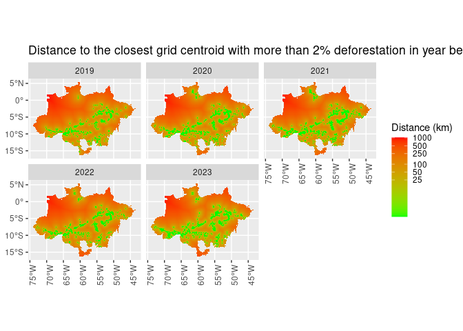
ggtitle(paste("Distance to the closest grid centroid with more than 2%",
"deforestation in year before"))def_sf %>%
ggplot() +
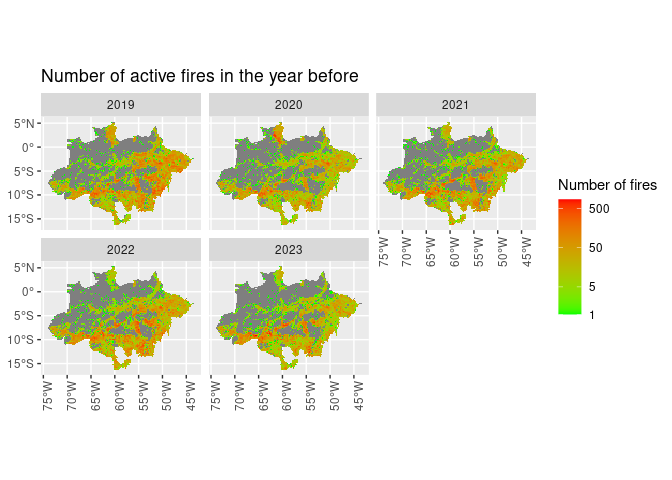
geom_sf(aes(fill = active_fires_ly), lwd = 0) +
scale_fill_gradient(name = "Number of fires",
trans = "log",
breaks = c(1, 5, 50, 500),
low = "green",
high = "red") +
facet_wrap(~ref_year) +
theme(axis.text.x = element_text(angle = 90)) +
ggtitle("Number of active fires in the year before")
#> Warning: Transformation introduced infinite values in discrete y-axis