
source code:
Tone mapping is not used in this version, since it will break the rule of energy conservation.
Build a real time renderer as a playground for learning about techniques on the PBRT book. And implement some materials described on the PBRT book (pure reflection, lambertian, microfacets ).
- OpenGL
- cuda 11
- Optix 7.4
One of the widely used BRDFs that describe microfacet is the Cook–Torrance BRDF. Cook-Torrance BRDF has both diffuse and specular parts:
where: $$ \begin{align} f_{lambert } &= \frac{albedo}{\pi}\ f_{cook-trrance}(\omega_o,\omega_i) &= \frac{D(\omega_h)F(\omega_i)G(\omega_i,\omega_o)}{4(\omega_i\cdot n)(\omega_o\cdot n)} \end{align} $$
-
**D **(Normal Distribution Function) : Estimates the number of microfacets oriented in the same direction as the half vector under the influence of surface roughness. T
-
F (Fresnel Equation) Fresnel equation: The Fresnel equation describes the ratio of light reflected by the surface under different surface angles.
-
G (Geometry Function): Describes the properties of the microfacet's self-shading. When a surface is relatively rough, the microfacet may block others and reduce the light reflected by the surface.
There are many specific implementation forms of D, F, and G functions. This implementation uses:
- D: Trowbridge-Reitz GGX
- F: Schlick's Fresnel approximation
- G:UE4's Schlick-GGX
The functions are as follows: $$ \begin{align} \alpha &= Roughness^2\ D(\boldsymbol{\omega}_h) &= \frac{\alpha^2}{\pi((\boldsymbol{n}\cdot \boldsymbol{\omega}_h)^2(\alpha^2-1)+1)^2}\ F( \boldsymbol{v},\boldsymbol{h}) &= F_0 + (1-F_0)2^{(-5.55473(\boldsymbol{v}\cdot \boldsymbol{h})-6.98316)(\boldsymbol{v}\cdot \boldsymbol{h})}\ k &= \frac{(Roughness+1)^2}{8}\ G_1(\boldsymbol{v}) &= \frac{\boldsymbol{n}\cdot \boldsymbol{v}}{(\boldsymbol{n}\cdot \boldsymbol{v})(1-k)+k}\ G(\boldsymbol{l},\boldsymbol{v})&=G_1({\boldsymbol{l}})G_1({\boldsymbol{v}}) \end{align} $$ The Fresnel equation used here is an accelerated version of Schlick's approximation.
-
D
D is the normal distribution function, which is a probability density function describing the probability density of the microfacet oriented.
Note : The relation between the
$\boldsymbol{\omega}_i$ and$\boldsymbol{h}$ is:$$ d\boldsymbol{\omega}_i = 4(\boldsymbol{\omega}_o\cdot \boldsymbol{\omega}_h)d\boldsymbol{\omega}_h$$
which is really important in importance sampling.
The prof of this relationship can be found in PBRT Ch. 14.11
-
F, G
There are a few subtleties involved with the Fresnel equation. One is that the Fresnel-Schlick approximation is only really defined for dielectric or non-metal surfaces. For conductor surfaces (metals), calculating the base reflectivity with indices(complex number) of refraction doesn't properly hold and we need to use a different Fresnel equation for conductors altogether. As this is inconvenient, we further approximate by pre-computing the surface's response at normal incidence (
$F_0$ ) at a 0 degree angle as if looking directly onto a surface. We interpolate this value based on the view angle, as per the Fresnel-Schlick approximation, such that we can use the same equation for both metals and non-metals.

interesting to observe here is that for all dielectric surfaces the base reflectivity never gets above 0.17
These specific attributes of metallic surfaces compared to dielectric surfaces gave rise to something called the metallic workflow. In the metallic workflow we author surface materials with an extra parameter known as metalness that describes whether a surface is either a metallic or a non-metallic surface.
We generally accomplish this as follows:
vec3 F0 = vec3(0.04);
F0 = mix(F0, surfaceColor.rgb, metalness)Because it is a probability density function itself, it is much more convenient for us to implement importance sampling.
- They are not probability density functions themselves, then we first need to obtain a probability density function requiring its integral value on the hemisphere to be 1
- Functions D, F, and G have different parameters. Function D needs to integrate the half vector direction
$\boldsymbol{\omega}_h$ , while functions F and G need to integrate the incident direction$\boldsymbol{\omega}_i$, so it is difficult to integrate the three at the same time.
We need to know
Since
$$
\begin{align}
& \int_{H^2}p(\boldsymbol{\omega}_i)d\boldsymbol(\omega)i = 1\
& \int{H^2}\cos \theta D(\boldsymbol{\omega}_h)d\boldsymbol{\omega}_h = 1
\end{align}
$$
We can get;
$$
\begin{align}
p(\boldsymbol{\omega}_i)d\boldsymbol(\omega)_i &= \cos \theta D(\boldsymbol{\omega}_h)d\boldsymbol{\omega}_h \
&= \cos \theta \sin \theta D(\theta,\phi)d\theta d\phi\
&= p_h(\theta,\phi)d\theta d\phi\
&= p_h(\theta)p_h(\phi)d\theta d\phi
\end{align}
$$
Since we know:
Got
$$
p_h(\theta)= \frac{2\alpha^2\cos \theta \sin \theta}{\pi((\boldsymbol{n}\cdot \boldsymbol{\omega}_h)^2(\alpha^2-1)+1)^2} = \frac{2\alpha^2\cos \theta \sin \theta}{\pi((\cos \theta)^2(\alpha^2-1)+1)^2}
$$
Then integrate
Sampling Completed!
D is the distribution of normals around the half vector NOT INCOMING VECTORS.
To convert it to incoming vector:
$$
p(\theta) = \frac{p_h(\theta_h)}{4(\boldsymbol{\omega}_o\cdot\boldsymbol{\omega}_h)}
$$
If we directly use D as PDF:
Fixed :

This non-linear mapping of monitors does output more pleasing brightness results for our eyes, but when it comes to rendering graphics there is one issue: all the color and brightness options we configure in our applications are based on what we perceive from the monitor and thus all the options are actually non-linear brightness/color options.
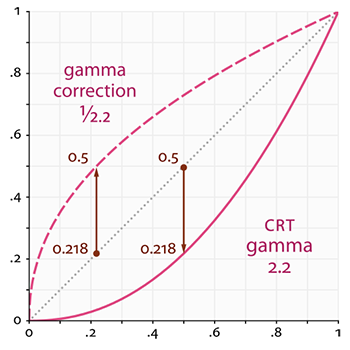
	const float gamma = 2.2;
    vec3 hdrColor = texture(u_Texture, TexCoord).rgb;
	finalColor = vec4(pow(hdrColor, vec3(1.0 / gamma)),1.0);
With out gamma correction, we will lose details at the bright areas of our scene

With gamma correction

This project is like a trainning plan for me to get better knowledge about PBRT. I learn how to implement PBRT based on this lightweight engine. At the same time hands-on porting and implementing the PBRT engine to my own system. I guess only when I can gradually port a more complex engine based on PBRT by myself can I say that I have truly mastered PBRT. This engine is the first step toward this target, although this project is still naive by now.
-
Implement BSSRDF
-
Add denoising with Spatiotemporal Variance-Guided Filtering (SVGF).
-
Increase the efficiency:
- The CPU occupation is about 50%-60%, transferring data between GPU and CPU twice per frame may bear significant responsibility for that.
- May be transplant the whole pipeline to Vulkan?
-
Implement Hair