The goal of the ccca package is to generate climate change conditioned advice for fisheries. Based on data inputs of a survey index time series, a catch time series and a climate change variable thought to affect stock production, a simple model is derived. The approach is emppirical in that it takes advantage of an empirically observed relationship between a stock’s surplus production and environmental or ecological variable even if the specific mechanism cannot be that well articulated. That is, there should be a hypothesis relating the E variables to surplus production but not necessarily an experimental body of evidence that supports it. By relaxing the necessary basis for evidence and casting this in a risk based framework, we are able to provide climate conditioned advice more immediately. This model is projected given climate scenarios that you provide using a built in function. This is done by fitting a normal distribution to your climate variable time series and then resamples it for a specified number of years into the future and for the number of Monte Carlo projection runs you want. You can shift the mean of this distribution or sample its quantiles to to simulate climate change. The variance of this distribution can also be altered to reflect the future climate scenario in terms of variance and not just mean. You can also easily develop your own scenario based on a different distribution, non-parametric resampling of the climate series or say a directional change in the climate variable, i.e. not a new stable state.
Various plotting functions are provided. You can find risk equivalent F strategies for a climate change scenario versus your baseline scenario. The contour plots show how the reference point risk changes with climate change. You can also determine climate conditioning factors to multiply the management tool (e.g. F, TAC) to condition the advice to climate change induced productivty changes in the tock and a risk equivalent fishing strategy.
The model was developed considering both density dependent and independent stock dynamics which are not very different for commerically exploited fish stocks.
The is work that is presently under consideration for primary literature. We please ask that you not try to publish other work based on this until the primary publication is out (it will be cited below). We are happy to take questions, comments and collaborate.
Gulf of St. Lawrence Greenland halibut also called turbot was used here as a case study. This is cold water seeking species which in the Gulf prefers depths >200m. It is also a stock which seems to be susceptible to relatively small changes in bottom water temperature and the growth rate of the stock seems closely related to bottom water temperature. This stock also has a good time series for the survey since 1990, landings and there are good temperature time series at relevant depths for the stock. There also is not a model for the stock. The data available for the stock is characterisitic for many Canadian fish and invertebrate stocks and because it is without a model, we label the situation as characteristic data moderate.
The objective considered here is a target objective. We setup a reference period (1995-2000) as a period when catches were good, relatively stable and the stock was healthy. Thus this is like a Bmsy target. A relative exploitation rate reference was developed from the same period. Because it is a target, by definition there is a 50% risk level for not achieving the target. This is essentially saying that for a target, the biomass will be above it 50% of the time and below it 50% of the time. We also set a period of 10 years as the maximum allowable time frame for achieving the objective which is largely a reflection of the population growth capacity for this particular stock.
Other biomass objectives and risk levels could also be chosen. For example a Blim might be represented by 40% of reference period biomass but it would also be necessary to decrease the risk tolerance for failure as well as the time period. So perhaps a risk level of 10% and time period of 5 years would be more appopriate for such an objective.
library(devtools)
install_github("duplisea/ccca")
library(ccca)
A default parameters file (params) comes with the package. It is a list with options needed to fit the P/B model and run projections. The mapply step just moves each list object into the global environment rather than calling the list element each time in Monte Carlo simulations so it is faster and it also does not alter the base parameterisation in the list so you can return to it later.
data(params)
mapply(assign, names(params), params, MoreArgs=list(envir = globalenv()))
Determine the annual P/B ratio of the population creating a dataframe with the index bumped by q
PB= PB.f(turbot, ref.years=ref.years, q=q)
Fit a relationship between the P/B and the E variable according to what you selected in params
PvsE= PBE.fit.f(PB,model.type=model.type, knots=knots, poly.degree=poly.degree)
Fit a normal distribution to the E time series and pull the parameters out.
Enorm= norm.fit.f(E=PB$E)
Edist.a=Enorm$estimate[1]
Edist.b=Enorm$estimate[2]
Develop the E projection values based on your choice of projection parameters
Eproj= Eprojnorm.f(Edist.a=Edist.a, Edist.b=Edist.b, Emean.shift=Emean.shift, proj.years=proj.years, N)
Develop the PB projection values based on the P/B vs E fit and the E projection you specified above. When add.residuals=1 then a residual is sampled for each time step of each projection and is added to the P/B values. If the P/B vs E fit is relatively unbiased then it will not make much difference to the median but it will increase the future uncertainty. If you set it =0 then the residual is not added and you will have less uncertainty in the future. If the P/B vs E model is biased, this bias will be more likely to be carried forward if residuals are not sampled (=0).
PBproj= PB.for.projection.f(PvsE=PvsE,Eproj,add.residuals=add.resids)
The fishing strategy. In this case is the the mean exploitation (Index corrected by catchability) during the last five years.
Fstrat= F.strategy(PB, 2014:2018, moratorium=F)
Run the projection given all the above calculations and parameters. The trajectory over the projection period and the probability that B is greater than the objective after the specified time range.
Bproj= projection.f(PB=PB, Bstart.mult=Bstart.mult, PBproj=PBproj, Fstrat, K=K, theta=1)
Fout= Fseq.f(PB,PBproj=PBproj,Fseq=fs,time.frame=time.frame, N=N, K=K)
PofF= PofF.f(PB,Fout,ref.pt=ref.pt)
Summarises the output of the projections by calculating quantiles and putting results in a dataframe. Calculates the probability of being at or above a reference point.
Bproj.summary= Bproj.summary.f(PB,Bproj,PBproj,Eproj)
P= rankprob.f(Bproj,PB,ref.pt)
We have done all of the above again but for different climate scenario mean shift, one warm and one cold, one with status quo mean temperature but increased variance and finally a null model run where P/B does not depend on E. It is not shown here but you do it by modifying the Emean.shift and Evariance parameters and re-running the above steps. These projection objects have names warm, cold, E.var.inc to distinguish them from the base run and they appear in the figures
Run mutliple simulations for each combination of E scenario and F. First the E and PB scenarios are set up and then multiple projections are made based on the exploitation rate series specified in the parameters file.
ECCF= Eproj.list.f(Emean.shifts=Emean.shifts, N=N.CCF, proj.years=proj.years, Edist.a=Edist.a,
  Edist.b=Edist.b)
PBCCF= PBproj.list.f(PvsE=PvsE, Eprojection=ECCF)
CCF.raw= P.R.for.EF.f(E.CCF=ECCF, PB.CCF=PBCCF, Fs=fs, PB=PB, ref.pt=ref.pt, Bstart.mult=Bstart.mult,
  K=K, theta=theta)
The plot of the Gulf of St Lawrence showing the main fishing areas for
turbot 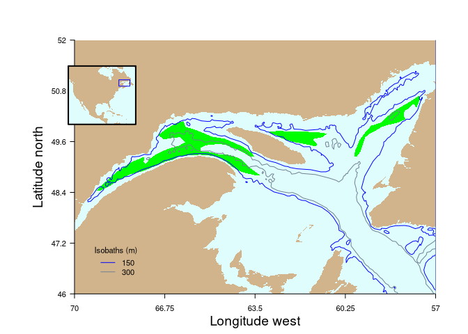
The basic data time series for the index, catch and E variable 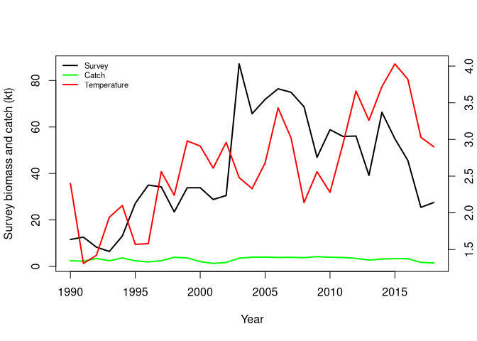
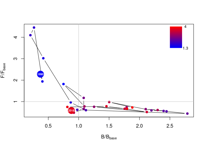
The Kobe plot of the historical data with the E variable colour coded on top of the points. There is function called Kobe.f to do this.
Kobe.f(PB=PB,E=PB$E)
colramp.legend(col1="red", col2="blue", ncol=length(PB$E), 2.5, 3.5, 2.7, 4.5)
The P/B vs E data plot and fitted model. 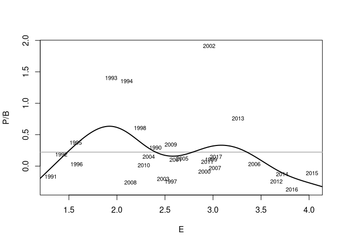
The normal distrubtion fitted to the E series which is sampled for
future climate projections altering the mean and variance for different
climate scenarios. 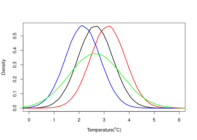
The distribution of the P/B values for the future projections. It is the
P/B that results by sampling E distribution function to simulate a
future climate and while altering the mean and variance if desired. The
P/B distribution is then deermined by running sampled E value through
the fitted P/B vs E relationship. 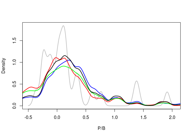
The plot of the projection given your E scenario for both density
independent and dependent models. The biomass reference level is
depicted as the horizontal dashed line. Confidence intervals are 90%.
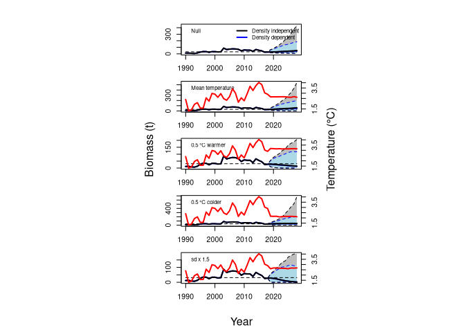
What is clear from the projections is that a decrease in temperature from the baseline is not good for the stock while an increase in temperature is certainly not good. What is more surprising is that even if mean temperature is the same as the baseline but there is an important increase in variance of the temperature, this is perhaps the worst case for the stock. There is a larger perentage of the P/B density <0 for the increased variance scenario than for any other scenario (Fig. 6). ___________________________________________
The probability that the biomass is greater than the reference level
each year of the projection. The horizontal dashed line represents the
risk tolerance of not achieving the objective. i.e. For the objective to
be met, the biomass line should be above the risk line at the end of the
time.frame period specified in the parameters list. 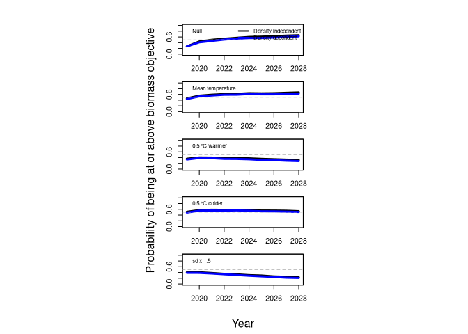
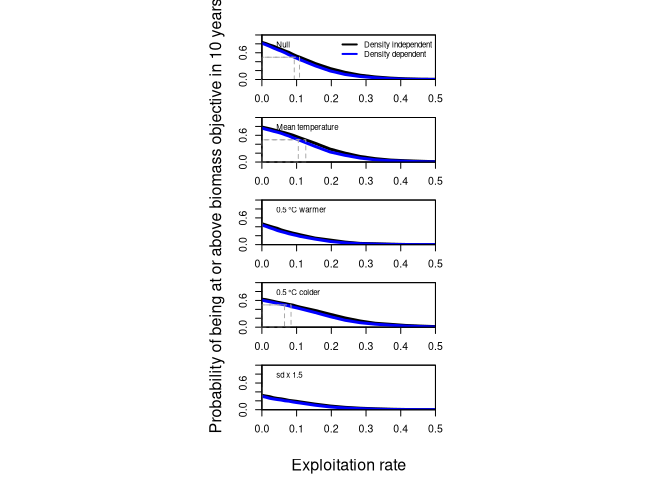
The maximum exploitation rate that will achieve the objective in the specified time period given the E scenario projected.
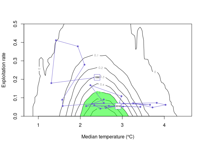
You can determine climate conditioning buffer factors from the contour plot (Fig 10) for the particular objective. So if the acceptable risk level is 50% (a target) then one can follow the 0.5 contour to see what the maximum exploitation rate could be for various future temperatures. The buffering factor would be the ratio of the long term mean temperature exploitation on the 50% risk contour with that at the proposed future temperature. The buffering factor is the incremental risk buffer. If one were interested in incremental risk of status quo fishing then they would plot the exploitation rate of long term mean temperature and status quo exploitation and determine on what risk contour it landed. Then do the same with the hypothesised future median temperature and status quo exploitation rate. The difference between the two risk levels is the incremental risk.
Incremental risk of assuming turbot production is affected by climate change vs not being affected can also be calculated by looking at how much the exploitation rate would need to change under one of the climate scenarios vs the null model. This incremental risk is the risk of assuming climate change is not important given your objective and future climate scenario.
The contour plot and climate conditioning factors essentially show the dependence of reference points on the environmental conditions. Ideally a reference point is relatively invariant to external factors but the reality is that none are. The domed contours over the temperature dimension esssentially show degree of variance caused by change in the environment and climate change in what are essentially dynamic reference points.
The DFO peer review group provided considerable feedback on these simulations. Mariano Koen-Alonso suggested that density dependence should be considered in these simulations.
Johanne Gauthier provided the turbot data and several temperature time series relevant to the turbot survey catches. Peter Galbraith provided several temperature and salinity E variables available in the turbot data object. Denis Gilbert provided the oxygen concentration and saturation levels for the deep water (>295 m) of the St Lawrence estuary.
DFO. 2018. Assessment of the Greenland Halibut stock in the Gulf of St. Lawrence (4RST) in 2017. DFO Can. Sci. Advis. Sec. Sci. Advis. Rep. 2018/035. http://waves-vagues.dfo-mpo.gc.ca/Library/40714007.pdf
Duplisea, D.E., Roux, M-J., Hunter, K.L. and Rice, J. 2019. Resource management under climate change: a risk-based strategy to develop climate-informed science advice. Can. Sci. Advis. Sec. Res. Doc. 2019/044. http://www.dfo-mpo.gc.ca/csas-sccs/Publications/ResDocs-DocRech/2019/2019_044-eng.html
Galbraith, P.S., Chassé, J., Nicot, P., Caverhill, C., Gilbert, D., Pettigrew, B., Lefaivre, D., Brickman, D., Devine, L., and Lafleur, C. 2015. Physical Oceanographic Conditions in the Gulf of St. Lawrence in 2014. DFO Can. Sci. Advis. Sec. Res. Doc. 2015/032. v + 82 p http://www.dfo-mpo.gc.ca/csas-sccs/Publications/ResDocs-DocRech/2015/2015_032-eng.html
Gilbert, D., B. Sundby, C. Gobeil, A. Mucci, G.-H. Tremblay 2005. A seventy-two-year record of diminishing deep-water oxygen in the St. Lawrence estuary: The northwest Atlantic connection. Limnology and Oceanography. 50: 1654-1666.
