Vehicle Detection Project
The goals / steps of this project are the following:
- Perform a Histogram of Oriented Gradients (HOG) feature extraction on a labeled training set of images and train a classifier Linear SVM classifier
- Optionally, you can also apply a color transform and append binned color features, as well as histograms of color, to your HOG feature vector.
- Note: for those first two steps don't forget to normalize your features and randomize a selection for training and testing.
- Implement a sliding-window technique and use your trained classifier to search for vehicles in images.
- Run your pipeline on a video stream (start with the test_video.mp4 and later implement on full project_video.mp4) and create a heat map of recurring detections frame by frame to reject outliers and follow detected vehicles.
- Estimate a bounding box for vehicles detected.
** Import the neccessary modules and data **
import matplotlib.image as mpimg
import matplotlib.pyplot as plt
% matplotlib inline
import numpy as np
import pickle
import cv2
import glob
from sklearn.preprocessing import StandardScaler
from importlib import reload
from sln import utils; reload(utils)
from sln import train; reload(train)
from sln import search; reload(search)
<module 'sln.search' from 'D:\\side\\CarND-Vehicle-Detection\\sln\\search.py'>
svc_pickle = pickle.load( open("svc.p", "rb" ))
svc = svc_pickle['svc']
scaler = svc_pickle['scaler']
Histogram of Oriented Gradients (HOG)
Explain how (and identify where in your code) you extracted HOG features from the training images.
The code I extract HOG features is contained in ./sln/train.py, the function get_hog_features (line 6-16).
I use the same parameters as the following example:
images = glob.glob('data/vehicles/*/*.png')
img = cv2.imread(images[np.random.randint(len(images))])
img = cv2.cvtColor(img, cv2.COLOR_BGR2RGB)
YCrCb = cv2.cvtColor(img, cv2.COLOR_RGB2YCrCb)
orient = 9
pix_per_cell = 8
cell_per_block = 2
hog_feat1, hog1_vis = train.get_hog_features(YCrCb[...,0], orient, pix_per_cell, cell_per_block, True)
hog_feat2, hog2_vis = train.get_hog_features(YCrCb[...,1], orient, pix_per_cell, cell_per_block, True)
hog_feat3, hog3_vis = train.get_hog_features(YCrCb[...,2], orient, pix_per_cell, cell_per_block, True)
plt.figure(figsize=(20,8))
plt.subplot(141)
plt.imshow(img)
plt.subplot(142)
plt.imshow(hog1_vis)
plt.subplot(143)
plt.imshow(hog2_vis)
plt.subplot(144)
plt.imshow(hog3_vis)
<matplotlib.image.AxesImage at 0x20227b9ae10>
Explain how you settled on your final choice of HOG parameters
After some experiments the color space used is YCrCb same as in the course since it does improve the training accuracy (see below).
Classifer
I trained a linear SVG using the feature vector combined with binned color, histograms of color and from YCrCb extacted vector.
The feature vector is normalized using sklearn.preprocessing.StandardScaler.
The training code is noted in the Jupyter notebook train.ipynb.
The classifier is able to score 0.9909 on the test set.
Sliding Window Search
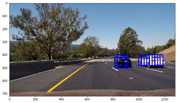
The sliding search is implemented in ./sln/search.py, the function find_cars (line 5-57). It returns a set of bounding boxes by predict the position where vehicles could be located.
To improve the efficiency of the efficiency of the detection and tracking, the HOG features at prediction time were taken once against an ROI of the image, rather than on independent windows.
I have tried different scale for the window. The scale beginning at 1.3 yields a satisfying result in the test image.
An example:
ystart = 400
ystop = 656
orient = 9
pix_per_cell = 8
cell_per_block = 2
scale = 1.3

img = mpimg.imread('test_images/test6.jpg')
bboxes = search.find_cars(img, svc, scaler,
                          ystart, ystop, orient, pix_per_cell, cell_per_block, scale)
draw_img = search.draw_bboxes(img, bboxes)
plt.figure(figsize=(20,6))
plt.imshow(draw_img)
<matplotlib.image.AxesImage at 0x202309850b8>
I threshold the heatmap to discard the false positives.
draw_img, heatmap = search.draw_result(img, bboxes, threshold=1, output_heatmap=True)
plt.figure(figsize=(10,6))
plt.subplot(121)
plt.imshow(draw_img)
plt.title('Car Positions')
plt.subplot(122)
plt.imshow(heatmap, cmap='hot')
plt.title('Heatmap')
<matplotlib.text.Text at 0x2022f9bf4a8>
Video Implementation
In the video processing pipeline I used a multipl-scale sliding window (sln/search.py line 117-124) at scales [1.3, 1,6, 2, 2.5, 3, 5, 7].
All bounding boxes predicted from the last three frames are collected to generate a heapmap for current frame. This heapmap is thresholded against the being used scales plus 1.
Discussion
There are still false positives in the video. It often fails at the region with complex texture. I consider training a classifer with a different dataset, refering more previous frames in the video pipeline, or trying the convolutional neural networks approach.


