Advanced Lane Finding Project

import numpy as np
import cv2
import matplotlib.pyplot as plt
import matplotlib.image as mpimg
%matplotlib inline

Camera Calibration

The calibration.py shows how to compute the distortion coefficients using OpenCV:

There are 9x6=48 point located on the chessboard. (line 13)
Assuming these object points in the world coordinates are (0,0,0), (1,0,0),...,(8,5,0), which lie on the plane z=0. (line 18)
I detect these point in image coordinates calling cv2.findChessboardCorners. (line 23)
The distortion coefficients can be computed by applying cv2.calibrateCamera to objpoints and imgpoints. (line 29)

import calibration
ret, mtx, dist, rvecs, tvecs = calibration.calibrate('camera_cal/calibration*.jpg')

The followings shows the original image compared with distortion correction applied:

img_file = 'camera_cal/calibration2.jpg'
img = cv2.imread(img_file)
img = cv2.cvtColor(img, cv2.COLOR_BGR2RGB)
undist = cv2.undistort(img, mtx, dist, None, mtx)
fig, ax = plt.subplots(1, 2, figsize=(20, 5))
ax[0].set_title('original')
ax[0].imshow(img)
ax[1].set_title('undistorted')
ax[1].imshow(undist)

<matplotlib.image.AxesImage at 0x273d0fe06d8>

Pipeline (single images)

Distortion correction

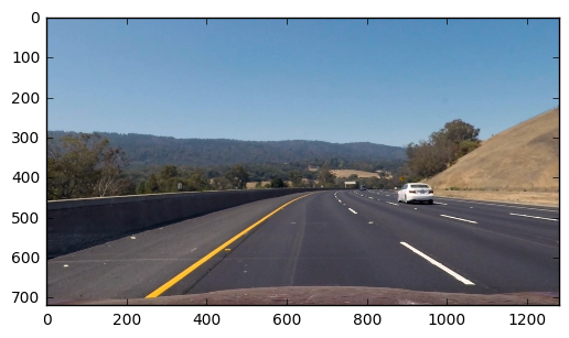
I apply the distortion correction to one of the test images like this one:

test_file = 'test_images/test3.jpg'
test_img = cv2.imread(test_file)
test_img = cv2.cvtColor(test_img, cv2.COLOR_BGR2RGB)
undist_test_img = cv2.undistort(test_img, mtx, dist, None, mtx)
plt.imshow(undist_test_img)

<matplotlib.image.AxesImage at 0x273d27f2d30>

Output the binary image

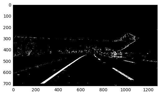
I combined the color transform and gradient filter and thresholded the output to generate the binary image. The functions are implented in ** process.py **, where:

undistort computes the distortion-corrected image with the previous parameters dist and mtx.
sobel_abs computes the the gradients in the horizontal/ vertical direction.
sobel_dir computes the the angle of the gradient
thresh computes the binary image by applying threshold to the previous outputs

The following shows a example ouput by combining the above mentioned functions:

from preprocess import undistort, sobel_abs, sobel_dir, thresh

filename = 'test_images/test3.jpg'
img = cv2.imread(filename)
undist_img = undistort(img, dist, mtx, is_BGR=True)

hls = cv2.cvtColor(undist_img, cv2.COLOR_RGB2HLS)
saturation = hls[...,2]
gray = cv2.cvtColor(undist_img, cv2.COLOR_RGB2GRAY)
gradx = sobel_abs(gray, (30,255), 5)
grady = sobel_abs(gray, (10,255), 5, (0,1))
sat_bin = thresh(saturation, (170,255))


combined = np.zeros_like(sat_bin)
cond = ( (sat_bin == 1) | ((gradx == 1) & (grady==1))  )
combined[cond] = 1
plt.imshow(combined, cmap='gray')

<matplotlib.image.AxesImage at 0x273d286bfd0>

Perspective transfom

Assuming the 4 points lie on the plane and the plane is flat, I chose the points as following:

Source	Destination
592, 452	294, 0
690, 452	1014, 0
1014, 659	1014, 720
294, 659	294, 720

from preprocess import pers_transform, src, dst

filename = 'test_images/straight_lines1.jpg'
img = cv2.imread(filename)
undist_straight = undistort(img, dist, mtx, is_BGR=True)


warp = cv2.warpPerspective(undist_straight, pers_transform, combined.shape[::-1], flags=cv2.INTER_LINEAR)

undist_img_drawn = np.copy(undist_straight)
cv2.polylines(undist_img_drawn, [src.astype(np.int32)], True, (255,0,255), 3)
warp_drawn = np.copy(warp)
cv2.polylines(warp_drawn, [dst.astype(np.int32)], True, (255,0,255), 3)
plt.figure(figsize=(20,6))
ax1 = plt.subplot(121)
ax1.imshow(undist_img_drawn)
ax2 = plt.subplot(122)
ax2.imshow(warp_drawn)

<matplotlib.image.AxesImage at 0x273d387fda0>

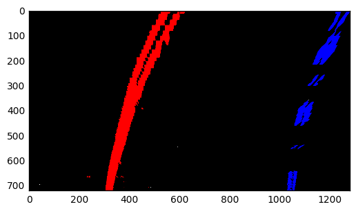
Fit the lane lines in the warped binary image

I took the code from the course with some modifications. I increased the searching windows and the searching width along with an early stopping condition.

The equation to fit to lines is quadratic polynomial:

With this modified window-sliding algorithm I fit my lane lines as following:

from lane_finding import slide_window

combined_warp = cv2.warpPerspective(combined, pers_transform, combined.shape[::-1], flags=cv2.INTER_LINEAR)

out, left, right, left_m, right_m = slide_window(combined_warp, draw=True)
plt.imshow(out)

<matplotlib.image.AxesImage at 0x273d3954a20>

Measuring curvature

where A,B are the coefficients of the fit quadratic polynomial.

from lane_finding import calculate_radii, calculate_deviation
y_bottom = 720
width = 1200
left_radius, right_radius = calculate_radii(y_bottom, left_m, right_m)
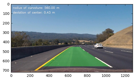
radius_curv = 0.5 * (left_radius + right_radius)

Deviation of the center

Assuming the camera is at the center of the car, I compute how far the center deviates from the center of lanes.

from lane_finding import calculate_deviation
deviation = calculate_deviation(y_bottom, width, left_m, right_m)

Mark the lane in the test image

from preprocess import pers_transform_inv
from lane_finding import draw_info_unwrap
result = draw_info_unwrap(undist_img, pers_transform_inv, left, right, radius_curv, deviation)
plt.imshow(result)

<matplotlib.image.AxesImage at 0x273d7736f98>

Pipeline (video)

The link to my video result

from moviepy.editor import VideoFileClip
from IPython.display import HTML
from process import Context

ctx = Context()

output = 'output_video.mp4'
project_clip = VideoFileClip("project_video.mp4")
output_clip = project_clip.fl_image(ctx.process)
output_clip.write_videofile(output, audio=False)

[MoviePy] >>>> Building video output_video.mp4
[MoviePy] Writing video output_video.mp4


100%|████████████████████████████████████████| 1261/1261 [00:59<00:00,  21.37it/s]


[MoviePy] Done.
[MoviePy] >>>> Video ready: output_video.mp4

Discussion

The difficulty is to recognize the yellow and white lane lines at the same time under different lighting condition. When there is shadow casting on the lane, many pixels at the edges of the shadow are recognized as the part the lane line, because I have applied thresholding to gradients. I mitigate this by reducing the searching range in the polynomial fitting stage. There could be a more robust approach where some specific line detectors are established to distiguish the line from the shadow considering different lighting condition.

ab1153 / CarND-Advanced-Lane-Lines