problem addressed: in-context learning on function classes, the ability of transformer models to learn contextual information when processing linear functions
Approach: Empirical Approach, train transformers from scratch and compare to the optimal least square estimator, sparse linear functions, two-layer neural networks, and decision trees.
In-context learning refers to the ability of a model to condition on a prompt sequence consisting of in-context examples (input-output pairs corresponding to some task) along with a new query input, and generate the corresponding output (without the need to perform any parameter updates after the model is trained).
Here a model in-context learn a function class F, for “most” functions f ∈ F, and approximate f(xquery) by conditioning on a prompt sequence (x1, f(x1),..., xi, f(xi), xquery) containing in-context examples and the query input.
Let Dx be a distribution over inputs in 20 dimensions, e.g. linear functions: isotropic Gaussian distribution N(0, Id), and DF be a distribution over functions in F, e.g. linear functions:the distribution over linear functions with weight vectors drawn from an isotropic Gaussian (N(0, Id), setting f(x) = w⊤x. Inputs xi and xquery, f are drawn i.i.d from their distributions over Dx and DF.
We say that a model M can in-context learn the function class F up to ε, with respect
to (DF , DX ), if it can predict f (xquery) with an average error
 where l(·, ·) is some appropriate loss function, such as the squared error.
question 2: How to evaluate the ability of the transformer model to generalize to unseen functions? hint: reflect on how we sample our input data.
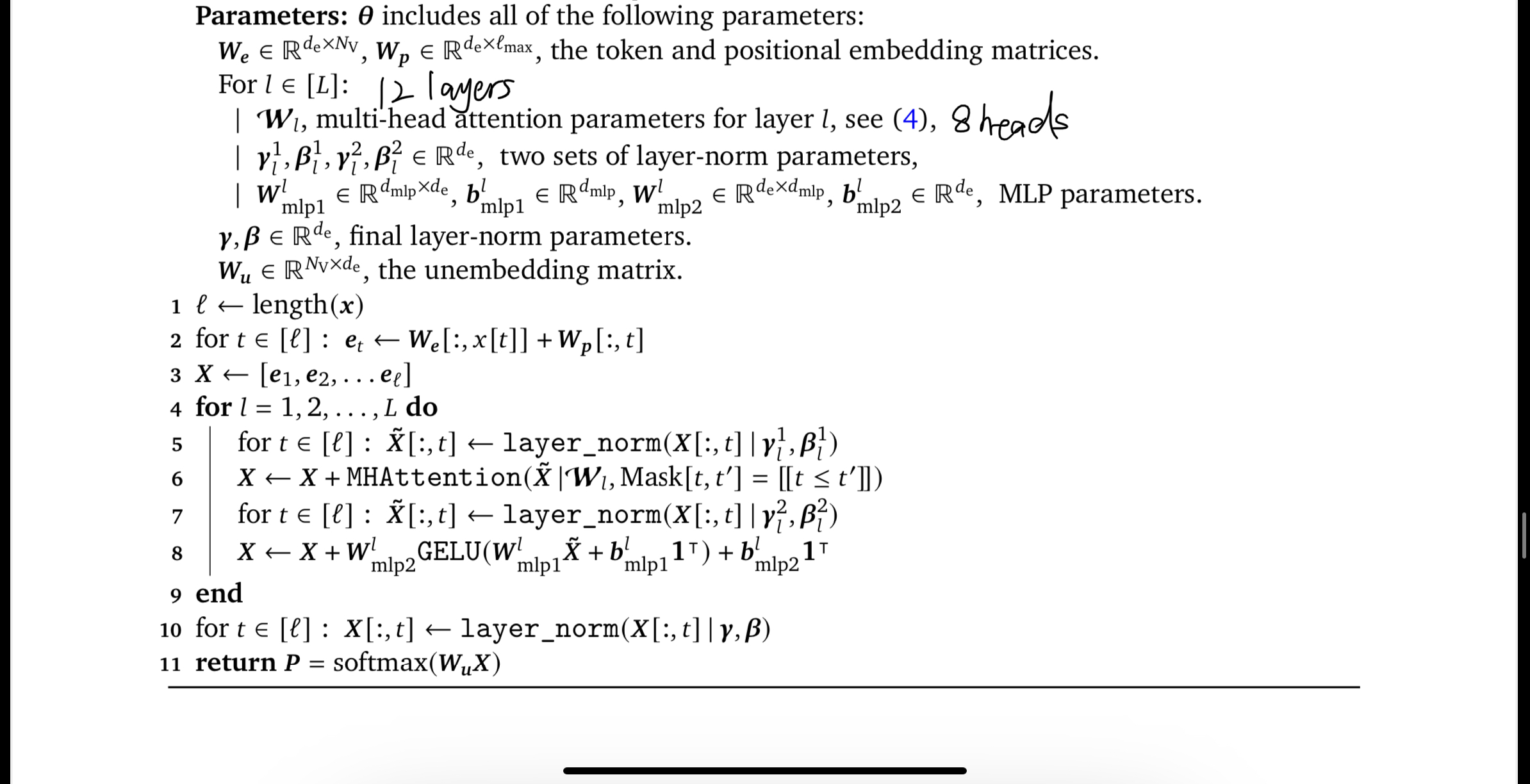
Model: decoder-only Transformer architecture from the GPT-2 family
Input: P =(x1,f(x1),x2,f(x2),...,xi,f(xi),xi+1)
Output: Mθ(xquery), a sequence of vectors then map the vector produced by the model to a scalar
Parameter: θ includes 12 layers and 8 heads
for each layer: forward pass: prediction of the model at the position corresponding to xi (that is absolute position 2i − 1) as the prediction of f(xi).
- step 1: at each training step, sampling a batch of prompt
- step 2: model Mθ aiming to minimize the expected loss over prompt, updating the model through a gradient update (we use a batch size of 64 and train for 500k total steps)
- step 3: compare with baseline: a)the least squares estimator, computing the minimum-norm linear fit to the in-context examples (xi, yi), (b) n-Nearest Neighbors, averaging the yi values for the n nearest neighbors of xquery, (c) averaging the values yixi to estimate w and compute the inner product of this estimate with xquery.
- result: the trained model achieves error comparable to the optimal least squares estimator,
- sampling prompt inputs or functions from a different distribution, that is Dtrain ̸= Dtest X/F X/F
- introducing a mismatch between in-context examples and the query input, that is Dtest result: the performance of our model is quite robust to such shifts, indicating that it has learned to perform linear regression with some generality.
Skewed covariance. We sample prompt inputs from N(0, Σ) where Σ is a skewed covariance matrix with eigenbasis chosen uniformly at random and ith eigenvalue proportional to 1/i2. The model matches the performance of least squares until k = 10, mimicking the sharp drop in the error in this regime, but its error plateaus afterwards (see Figure 4a). Thus, it is not perfectly robust to this distribution mismatch but still does relatively well, achieving less than half the error of the nearest neighbor baseline in most cases.
Noisy linear regression. We add noise to each prompt output, that is, the ith output is equal to wT xi + εi where εi ∼ N(0, 1). The trained model closely tracks the performance of least squares when the number of in-context examples is not close to the input dimension 20 (see Figure 4b). Interestingly, the model also exhibits the double descent error curve [Belkin et al., 2019] that is known to manifest for the least squares estimator [Nakkiran, 2019]. Note that in this noisy setting, the optimal estimator corresponds to solving least squares with appropriate l2-regularization. However, since the model was trained on noiseless data, we cannot expect it to learn this.
What the article overlooked: While the paper does not provide any explanation for why transformers exhibit such capabilities to compute the value of that function given an input in the context. There's a lot of mentioning for 'in-context'. All the model is doing is doing sequential modeling that given a series of inputs and the corresponding function values, the model predicts the function value of the previous input.
What can be developed more: More complex function classes than sparse linear functions, two-layer neural networks, and decision trees. More distribution shift


