Last updated: 2023-02-13
| CI | Development | CRAN | License |
|---|---|---|---|
 |
 |
Species-habitat associations in R is a R package to
analyze species-habitat associations. Therefore, information about the
location of the species is needed (as a point pattern) and about the
environmental conditions (as a raster map). In order to analyse the data
for significant habitat associations either the location data or the
environmental data is randomized n-times. Then, counts within the
habitats are compared between the randomized data and the observed data.
Positive or negative associations are present if the observed counts is
higher or lower than the randomized counts (using quantile thresholds).
Methods are described in Plotkin et al. (2000), Harms et al. (2001) and
Wiegand & Moloney (2014). shar is mainly based on the
spatstat (Baddeley et al. 2015) and
terra (Hijmans 2022) package.
The shar package is part of our academic work. To cite the package or acknowledge its use in publications, please cite the following paper.
Hesselbarth, M.H.K., (2021). shar: A R package to analyze species-habitat associations using point pattern analysis. Journal of Open Source Software, 6(67), 3811. https://doi.org/10.21105/joss.03811
The get a BibTex entry, please use citation("shar").
You can install the released version of shar from CRAN with:
install.packages("shar")And the development version from GitHub with:
# install.packages("remotes")
remotes::install_github("r-spatialecology/shar")
This also automatically installs all non-base R package dependencies,
namely the following packages: classInt, raster, spatstat.explore,
spatstat.model, spatstat.geom.
library(shar)
library(spatstat)
library(terra)

set.seed(42)
shar comes with build-in example data sets. species_a and
species_b are exemplary location of species, e.g. trees, as
ppp-objects from the spatstat package. landscape contains
exemplary continuous environmental data. However, all methods depend on
discrete data. Therefore we need to classify the data first. However,
all methods require “fully mapped data” in a sense that NA cells of the
environmental data are allowed only if simultaneously these areas cannot
accommodate any locations of the point pattern (e.g., a water body
within a forest area). This needs to be reflected in the observation
window of the point pattern. For the torus translation method, no NA
values are allowed at all.
landscape_classified <- classify_habitats(raster = terra::rast(landscape), n = 5, style = "fisher")There are two possibilities to randomize the environmental data, both described in Harms et al. (2001). The first shifts the habitat map in all 4 cardinal directions around a torus. The second one assigns the habitat values to an empty map using a random walk algorithm. Both functions return a list with randomized rasters and the observed one. For more information on the methods, please click here.
torus_trans <- translate_raster(raster = landscape_classified)

random_walk <- randomize_raster(raster = landscape_classified, n_random = 39)
To plot the randomized raster, you can use the plot function and specify the number of raster as as well as the color palette used for the discrete environmental data.
col_palette <- c("#440154FF", "#3B528BFF", "#21908CFF", "#5DC863FF", "#FDE725FF")

plot(torus_trans, n = 3, col = col_palette)
To randomize the point pattern, either use the Gamma test described by Plotkin et al. (2000) or pattern reconstruction (Kirkpatrick et al. 1983; Tscheschel & Stoyan 2006).
gamma_test <- fit_point_process(pattern = species_b, process = "cluster", n_random = 39)

# (this can takes some time)
reconstruction <- reconstruct_pattern(pattern = species_b, n_random = 39, e_threshold = 0.05)
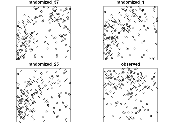
Of course, there are several utility functions. For example, you can
plot the summary function of the observed pattern and the simulation
envelopes of randomized patterns (what = "sf") or some randomized and
the observed pattern (what = "pp") using the plot function.
plot(reconstruction, what = "pp")Another utility function allows to calculate the differences between the observed pattern and the randomized patterns (also called energy using summary functions).
calculate_energy(reconstruction, return_mean = TRUE)
## [1] 0.04907375
The data was created that species_a has a negative association to
habitat 4 and species_b has a positive association to habitat 5, which
is reflected in the results.
Given the characteristics of the method, a positive association to one habitat inevitably leads to a negative association to at least one of the other habitats (and vice versa; Yamada et al. 2006). For example, a high amount of individual points in the positively associated habitat simultaneously mean that less individual points can be present in the other habitats.
Furthermore, please be aware that due to the randomization of the null
model data, results might slightly differ between different
randomization approaches (e.g., fit_point_process()
vs. translate_raster()) and even for repetitions of the same approach.
Thus, the exact lo and hi thresholds might be slightly different
when re-running the examples. However, the counts of the observed data
should be identical, and general results and trends should be similar.
significance_level <- 0.01

results_habitat_association(pattern = species_a, raster = torus_trans, significance_level = significance_level)
## > Input: randomized raster
## > Quantile thresholds: negative < 0.005 || positive > 0.995
##   habitat breaks count lo hi significance
## 1       1     NA    35 10 35         n.s.
## 2       2     NA    44 19 53         n.s.
## 3       3     NA    36 15 49         n.s.
## 4       4     NA     4 15 58     negative
## 5       5     NA    73 48 90         n.s.

results_habitat_association(pattern = reconstruction, raster = landscape_classified, significance_level = significance_level)
## > Input: randomized pattern
## > Quantile thresholds: negative < 0.005 || positive > 0.995
##   habitat breaks count    lo    hi significance
## 1       1     NA     6  2.19 13.43         n.s.
## 2       2     NA    18 17.57 55.86         n.s.
## 3       3     NA    18 33.19 58.00     negative
## 4       4     NA    21 35.38 54.81     negative
## 5 5 NA 129 37.38 84.10 positiveContributions to shar are highly welcomed and appreciated. This includes any form of feedback, bug reports, feature requests/suggestions, or general questions about the usage.
Please note that the shar package is released with a Contributor Code of Conduct. By contributing to this project, you agree to abide by its terms.
To contribute to this project, please see the Contributing guidelines.
Baddeley, A., Rubak, E., Turner, R., 2015. Spatial point patterns: Methodology and applications with R. Chapman and Hall/CRC Press, London. ISBN 978-1-4822-1020-0
Harms, K.E., Condit, R., Hubbell, S.P., Foster, R.B., 2001. Habitat associations of trees and shrubs in a 50-ha neotropical forest plot. Journal of Ecology 89, 947–959. https://doi.org/10.1111/j.1365-2745.2001.00615.x
Hijmans, R.J., 2022 terra: Spatial Data Analysis. R package version 1.6-7. https://CRAN.R-project.org/package=terra.
Kirkpatrick, S., Gelatt, C.D.Jr., Vecchi, M.P., 1983. Optimization by simulated annealing. Science 220, 671–680. https://doi.org/10.1126/science.220.4598.671
Plotkin, J.B., Potts, M.D., Leslie, N., Manokaran, N., LaFrankie, J.V., Ashton, P.S., 2000. Species-area curves, spatial aggregation, and habitat specialization in tropical forests. Journal of Theoretical Biology 207, 81–99. https://doi.org/10.1006/jtbi.2000.2158
Tscheschel, A., Stoyan, D., 2006. Statistical reconstruction of random point patterns. Computational Statistics and Data Analysis 51, 859–871. https://doi.org/10.1016/j.csda.2005.09.007
Wiegand, T., Moloney, K.A., 2014. Handbook of spatial point-pattern analysis in ecology. Chapman and Hall/CRC Press, Boca Raton. ISBN 978-1-4200-8254-8
Yamada, T., Tomita, A., Itoh, A., Yamakura, T., Ohkubo, T., Kanzaki, M., Tan, S., Ashton, P.S., 2006. Habitat associations of Sterculiaceae trees in a Bornean rain forest plot. Journal of Vegetation Science 17, 559–566. https://doi.org/10.1111/j.1654-1103.2006.tb02479.x

