openair is an R package developed for the purpose of analysing air quality data - or more generally atmospheric composition data. The package is extensively used in academia, the public and private sectors. The project was initially funded by the UK Natural Environment Research Council (NERC), with additional funds from Defra. The most up to date information on openair can be found in the package itself and the manual which provides an introduction to R with a focus on air quality data as well as extensive reproducible examples. An archive of newsletters in also available at the same location.
The current newsletter (Issue 18) summarises some of the recent changes to the package and is available here.
Installation of openair from GitHub is easy using the devtools package. Note, because openair contains C++ code a compiler is also needed. For Windows - for example, Rtools is needed.
require(devtools)
install_github('davidcarslaw/openair')
I also try to keep up to date versions of the package here if you can't build the package yourself.
openair has developed over several years to help analyse atmospheric composition data; initially focused on air quality data.
This package continues to develop and input from other developers would be welcome. A summary of some of the features are:
- Access to data from several hundred UK air pollution monitoring
sites through the
importAURNandimportKCLfunctions as well as archive data from the EEA (European Environment Agency) Airbase database. - Utility functions such as
timeAverageandselectByDateto make it easier to manipulate atmospheric composition data. - Flexible wind and pollution roses through
windRoseandpollutionRose. - Flexible plot conditioning to easily plot data by hour or the day,
day of the week, season etc. through the openair
typeoption available in most functions. - More sophisticated bivariate polar plots and conditional probability functions to help characterise different sources of pollution. A paper on the latter is available here.
- Access to NOAA Hysplit pre-calculated annual 96-hour back trajectories and many plotting and analysis functions e.g. trajectory frequencies, Potential Source Contribution Function and trajectory clustering.
- Many functions for air quality model evaluation using the
flexible methods described above e.g. the
typeoption to easily evaluate models by season, hour of the day etc. These include key model statistics, Taylor Diagram, Conditional Quantile plots.
It is easy to import hourly data from 100s of sites and to import several sites at one time and several years of data.
kc1 <- importAURN(site = "kc1", year = 2011:2012)
> head(kc1)
                 date o3 no2  co so2 pm10 nox no pm2.5 nv2.5 v2.5 nv10 v10  ws    wd                 site
1 2011-01-01 00:00:00 14  38 0.2   5   40  44  4    39    32    7   32   8 1.1 266.7 London N. Kensington
2 2011-01-01 01:00:00 28  29 0.2   3   36  38  6    30    24    6   29   7 1.2 271.9 London N. Kensington
3 2011-01-01 02:00:00 18  31 0.2   3   31  32  1    31    23    8   24   7 1.5 276.3 London N. Kensington
4 2011-01-01 03:00:00 14  29 0.2   3   31  31  1    29    21    8   23   8 2.1 278.7 London N. Kensington
5 2011-01-01 04:00:00 16  29 0.2   3   29  31  1    25    19    6   21   8 2.7 289.6 London N. Kensington
6 2011-01-01 05:00:00 24  27 0.1   3   25  29  1    23    16    7   18   7 2.8 303.6 London N. Kensington
  code
1  KC1
2  KC1
3  KC1
4  KC1
5  KC1
6 KC1Using the selectByDate function it is easy to select quite complex
time-based periods. For example, to select weekday (Monday to Friday)
data from June to September for 2012 and for the hours 7am to 7pm
inclusive:
sub <- selectByDate(kc1, day = "weekday", year = 2012, month = 6:9, hour = 7:19)
> head(sub)
                     date o3 no2   co so2 pm10 nox no pm2.5 nv2.5 v2.5 nv10 v10  ws    wd
12416 2012-06-01 07:00:00 24  23 0.23   3    6  36  9    21    14    7    5   1 1.4 307.4
12417 2012-06-01 08:00:00 34  21 0.23   3    9  33  7    NA    NA   NA    8   1 1.6 313.6
12418 2012-06-01 09:00:00 52  19 0.23   3    6  23  2    NA    NA   NA    3   3 1.6 330.0
12419 2012-06-01 10:00:00 62  13 0.23   3    7  17  2    NA    NA   NA    4   3 1.5 348.9
12420 2012-06-01 11:00:00 70  13 0.23   3    9  17  2    14     7    7    6   3 1.4 181.1
12421 2012-06-01 12:00:00 78  19 0.23   3    8  21  1    13     7    6    4   4 1.6   2.9
                      site code
12416 London N. Kensington  KC1
12417 London N. Kensington  KC1
12418 London N. Kensington  KC1
12419 London N. Kensington  KC1
12420 London N. Kensington  KC1
12421 London N. Kensington  KC1
Similarly it is easy to time-average data in many flexible ways. For example, 2-week means can be calculated as
sub2 <- timeAverage(kc1, avg.time = "2 week")One of the key aspects of openair is the use of the type option,
which is available for almost all openair functions. The type option
partitions data by different categories of variable. There are many
built-in options that type can take based on splitting your data by
different date values. A summary of in-built values of type are:
- "year" splits data by year
- "month" splits variables by month of the year
- "monthyear" splits data by year and month
- "season" splits variables by season. Note in this case the user can
also supply a
hemisphereoption that can be either "northern" (default) or "southern" - "weekday" splits variables by day of the week
- "weekend" splits variables by Saturday, Sunday, weekday
- "daylight" splits variables by nighttime/daytime. Note the user must
supply a
longitudeandlatitude - "dst" splits variables by daylight saving time and non-daylight saving time (see manual for more details)
- "wd" if wind direction (
wd) is availabletype = "wd"will split the data up into 8 sectors: N, NE, E, SE, S, SW, W, NW.
If a categorical variable is present in a data frame e.g. site then
that variables can be used directly e.g. type = "site".
type can also be a numeric variable. In this case the numeric
variable is split up into 4 quantiles i.e. four partitions
containing equal numbers of points. Note the user can supply the
option n.levels to indicate how many quantiles to use.
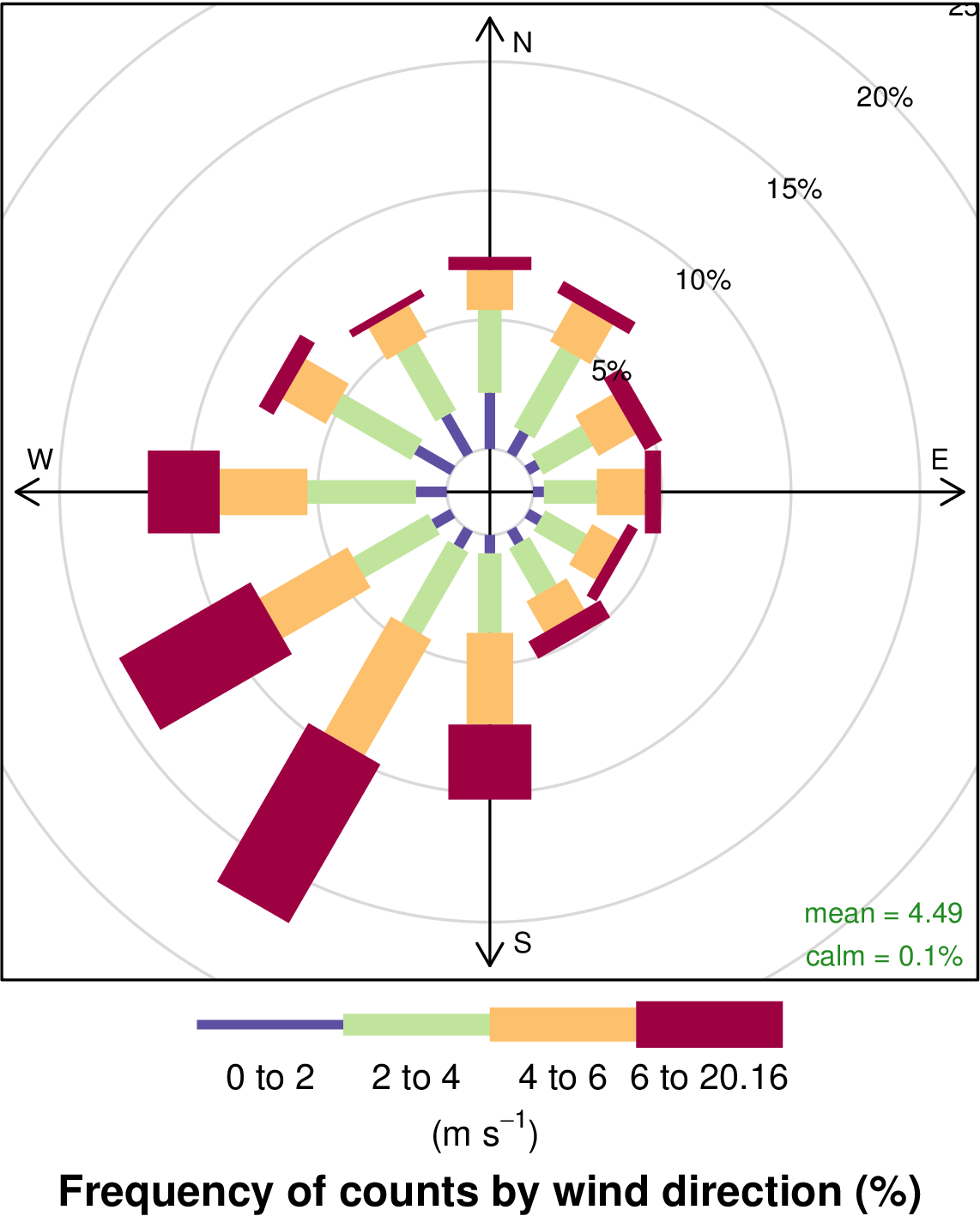
openair can plot basic wind roses very easily provided the variables
ws (wind speed) and wd (wind direction) are available.
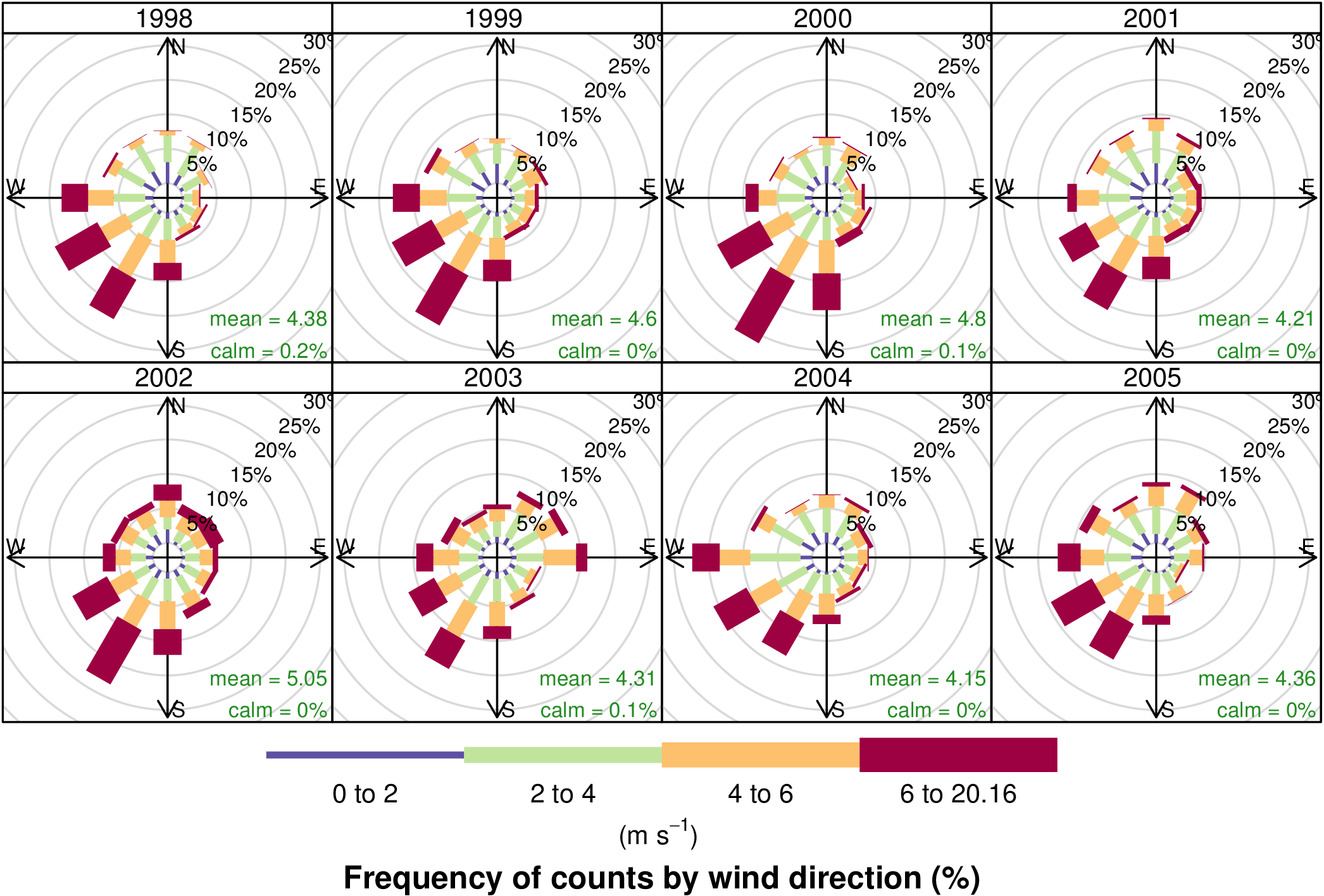
windRose(mydata)However, the real flexibility comes from being able to use the type option.
windRose(mydata, type = "year", layout = c(4, 2))

