Xunius / gplot

A Python module for creating quick and easy 2D geographical plots

GPlot -- a wrapper of matplotlib, cartopy and basemap for quick and easy geographical plots

Install

Install using conda:

conda install -c guangzhi gplot

Basic usage

The signature of the main plotting interfacing function is:

from gplot import plot2
plot2(var, method, ax, xarray=x, yarray=y)

where:

• var is np.ndarray, what to plot.
• method is a plotting method object, how to plot, e.g. Isofill which is contourf, Boxfill which is imshow, Quiver which is quiver plots.
• ax: matplotlib.Axes object, where to plot.
• xarray and yarray: x- and y- coordinate.

Examples

Default contourf plot of surface pressure, using basemap

import gplot
figure = plt.figure(figsize=(12, 10), dpi=100)
ax = figure.add_subplot(111)
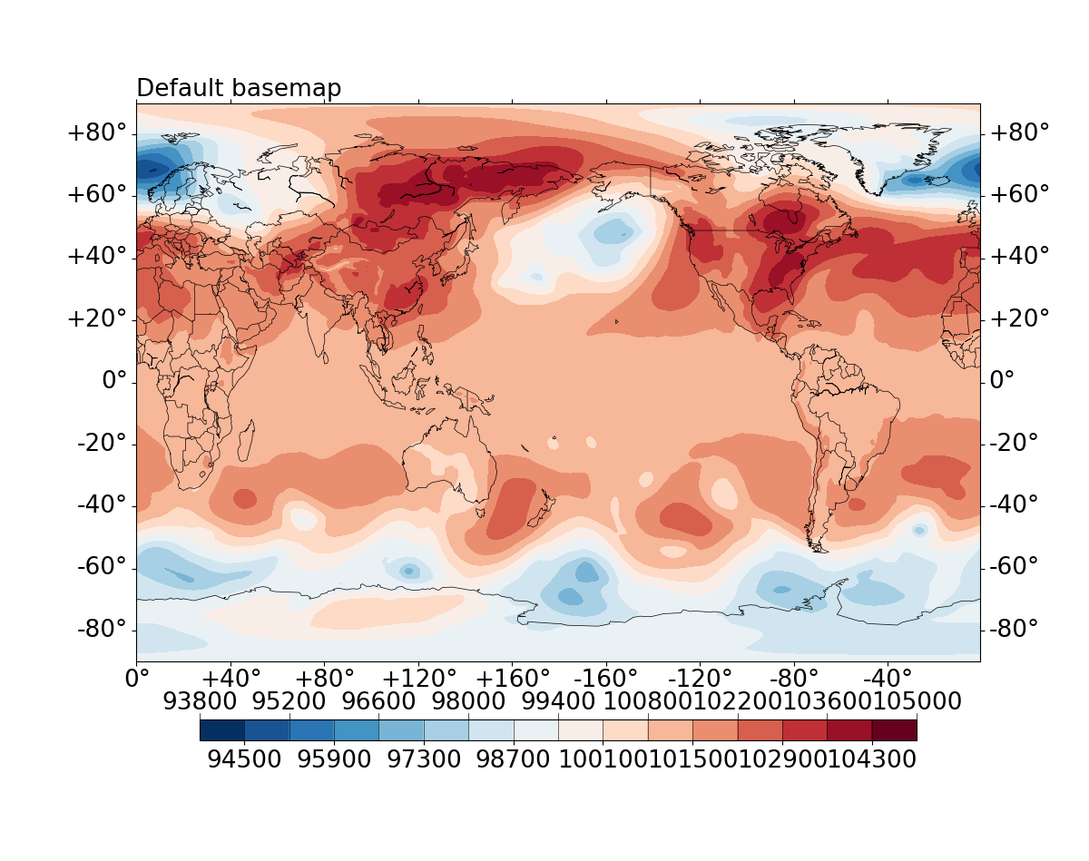
iso = gplot.Isofill(var)
gplot.plot2(var, iso, ax, xarray=lons, yarray=lats,
	title='Default basemap', projection='cyl',
	nc_interface='netcdf4')
figure.show()

Default contourf plot of global surface pressure field (in Pa), from ERA-I.

where var, lons and lats can be obtained, for instance, via netcdf4:

fin = netcdf4.Dataset(DATA_FILE_NAME, 'r')
var = fin.variables['msl'][:]
lons = fin.variables['longitude']
lats = fin.variables['latitude']

Currently, netCDF file reading using netcdf4 and CDAT are supported, iris and xarray are planned.

Control the number of contourf levels and overflow

import gplot
figure = plt.figure(figsize=(12, 10), dpi=100)
ax = figure.add_subplot(111)
iso = gplot.Isofill(var, num=10, zero=1, split=1,
                    min_level=11000, qr=0.01)
gplot.plot2(
    var, iso, ax, xarray=lons, yarray=lats,
    title='Isofill with overflows', projection='cyl',
    nc_interface='netcdf4')
figure.show()

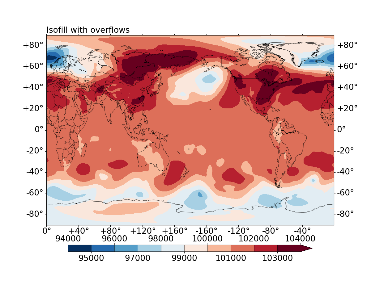
Contourf plot of global surface pressure field (in Pa), from ERA-I. Control the number of contourf levels and set overflow levels on both ends.

where:

• num = 10 specifies the desired number of contourf levels.
• zero = 1: 0 is allowed to be one of the contourf levels.
• split = 1: split a divergence colorbar if the plotted data has both positive and negative values.
• min_level = 11000: desired minimum level of the contourf levels.
• qr = 0.01: desired maximum level of the contourf levels, specified by the 0.01 right quantile.

Multiple subplots sharing a same colorbar

import gplot
figure, axes=plt.subplots(figsize=(12,10), nrows=2, ncols=2, constrained_layout=True)
plot_vars=[var[ii] for ii in range(4)]
iso=gplot.Isofill(plot_vars, ql=0.005, qr=0.001)
titles=['var-%d' %ii for ii in range(4)]

for ii, vii in enumerate(plot_vars):
ax=axes.flat[ii]
gplot.plot2(vii, iso, ax, title=titles[ii], legend='global', projection='cyl')

figure.show()

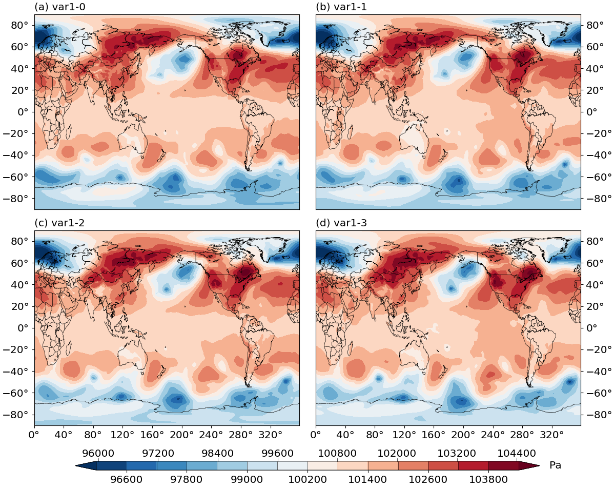
Contourf plot of global surface pressure field (in Pa), from ERA-I. The 4 subplots are sharing the same colorbar.

More examples are given in the tests subfolder

Documentation

More detailed documentation can be found at: https://gplot.readthedocs.io/en/latest/

Dependencies

• Python>=3
• numpy
• matplotlib
• scipy
• netcdf4
• basemap (note that for usage with basemap, needs matplotlib<=3.2.2) or cartopy (WIP)
• (optional) CDAT

Contributing and getting help

This package is still in early alpha.

We welcome contributions from the community. Please create a fork of the project on GitHub and use a pull request to propose your changes. We strongly encourage creating an issue before starting to work on major changes, to discuss these changes first.