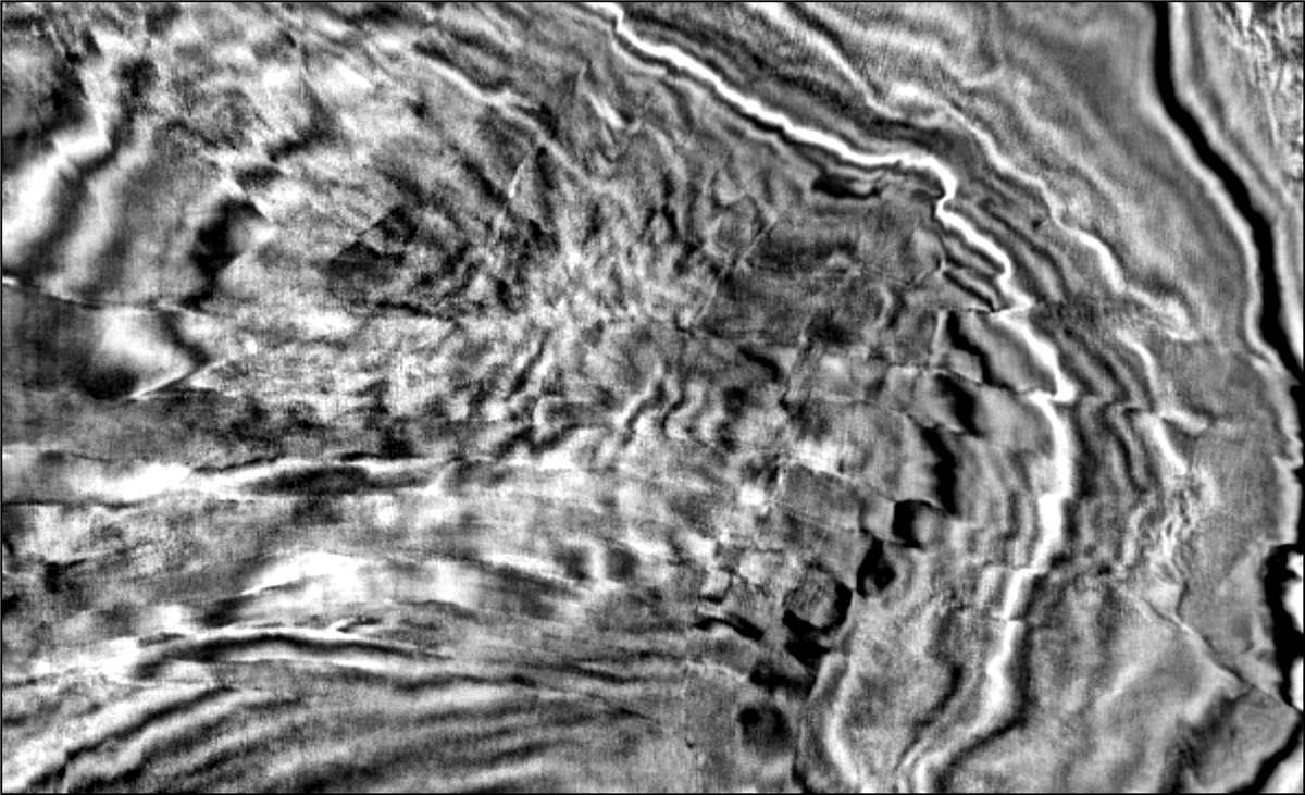
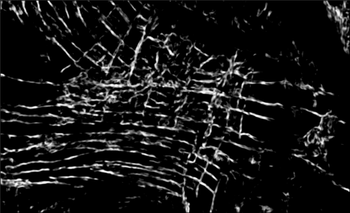
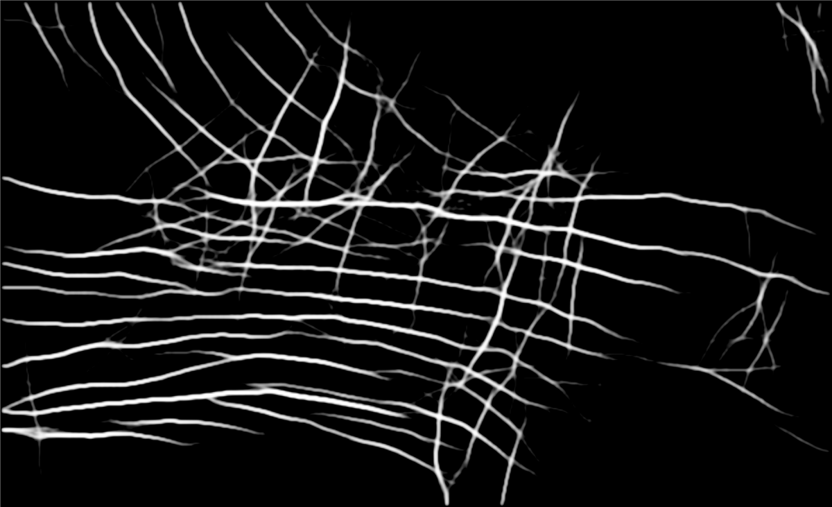
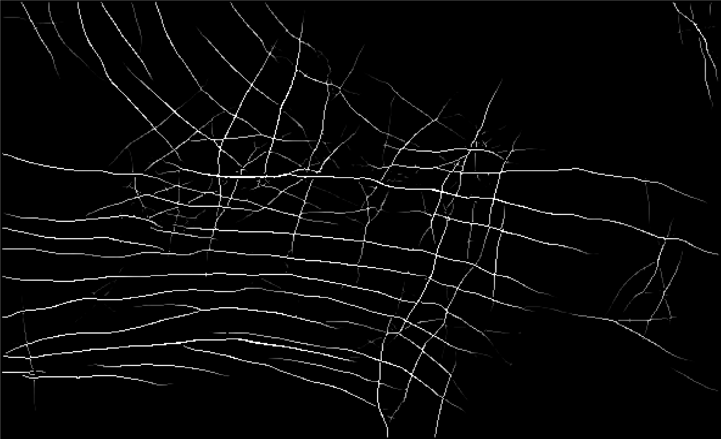
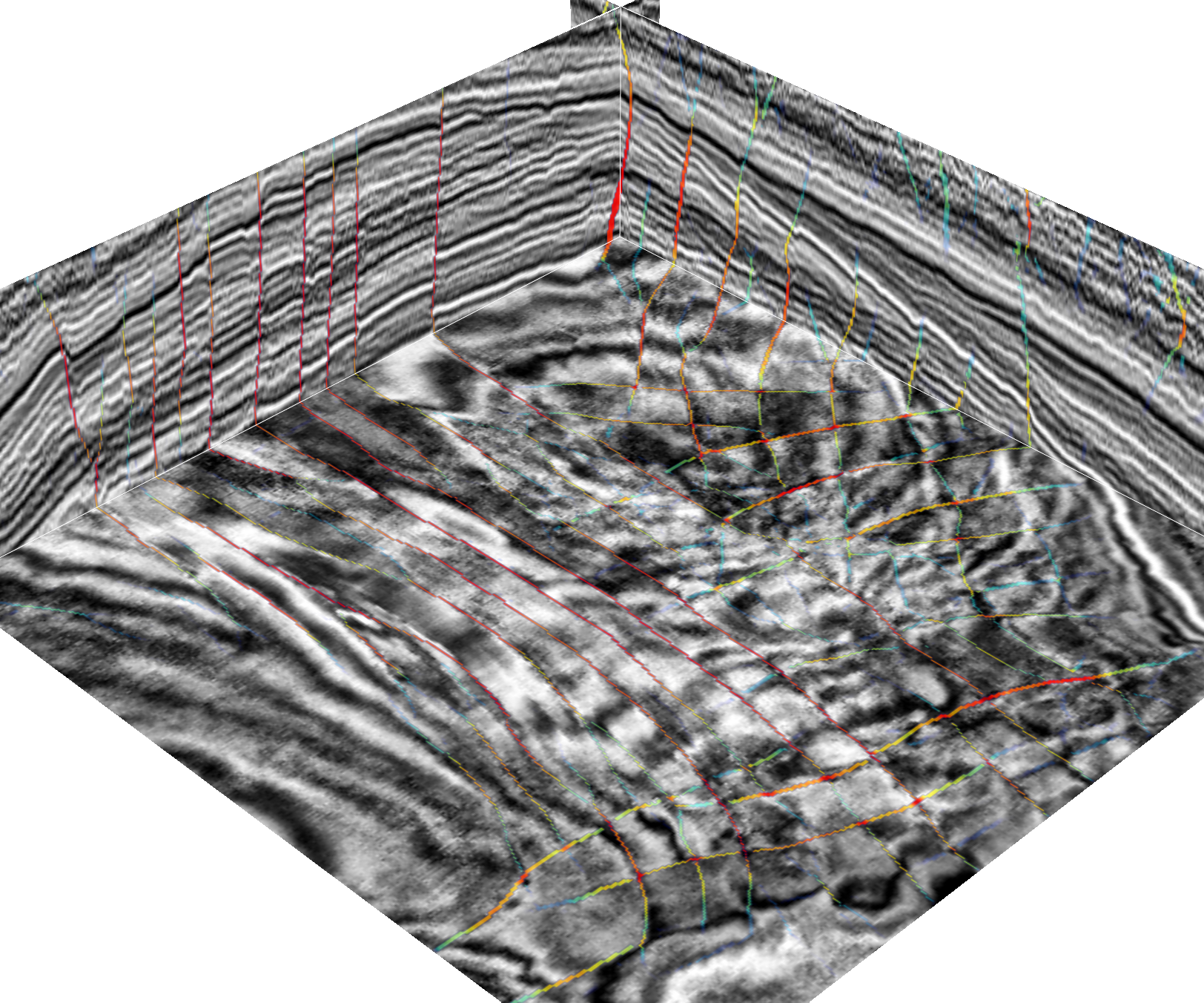
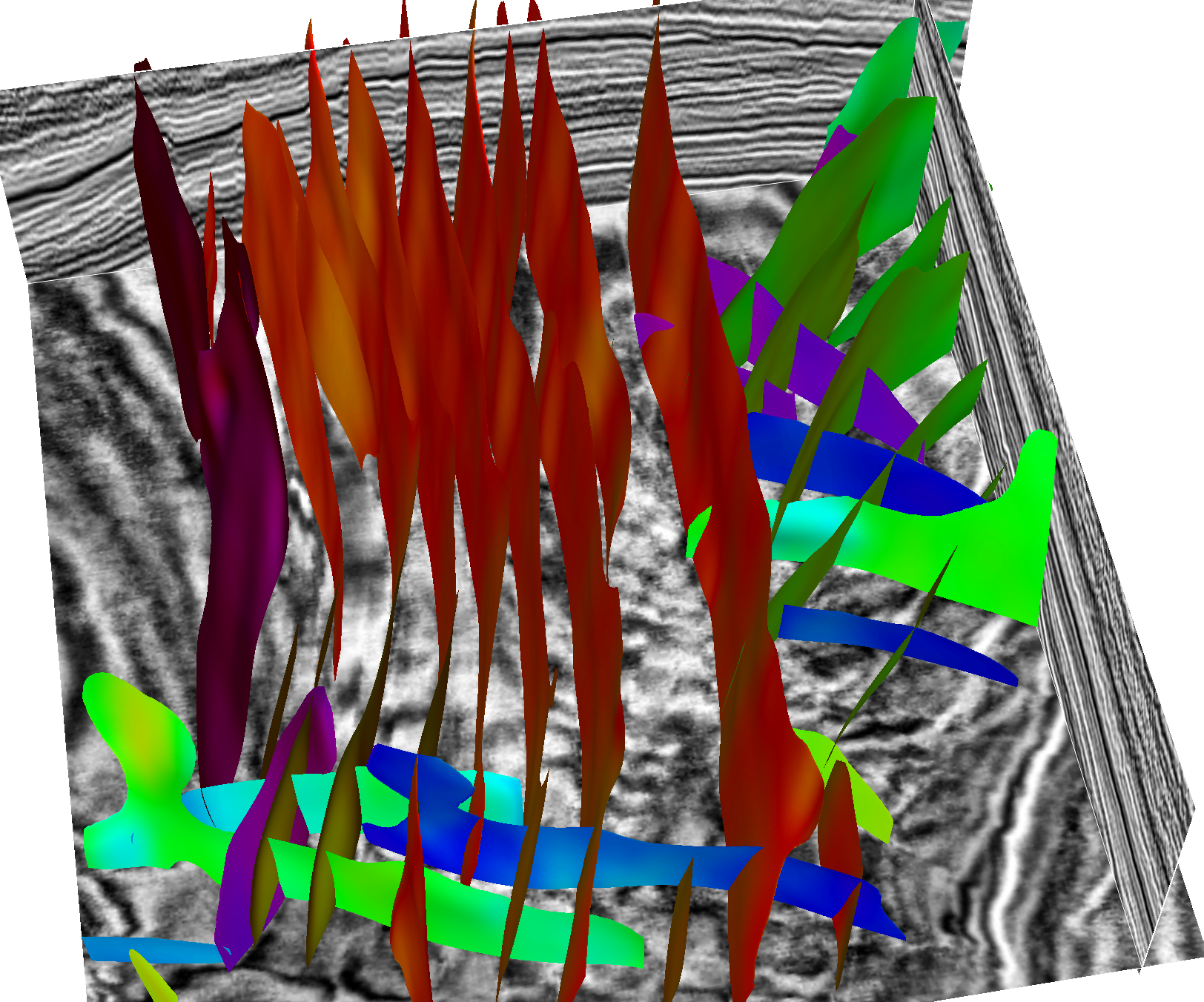
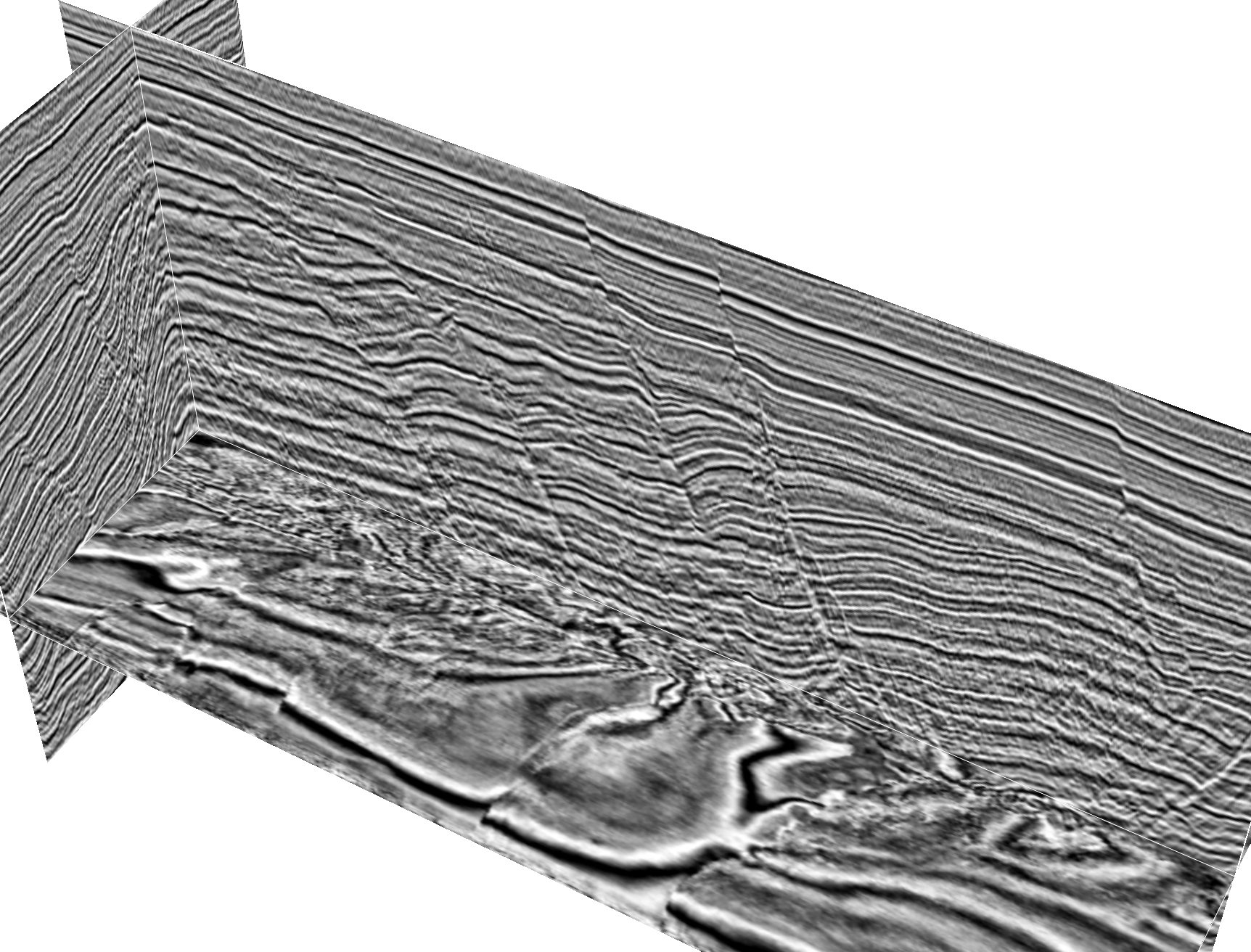
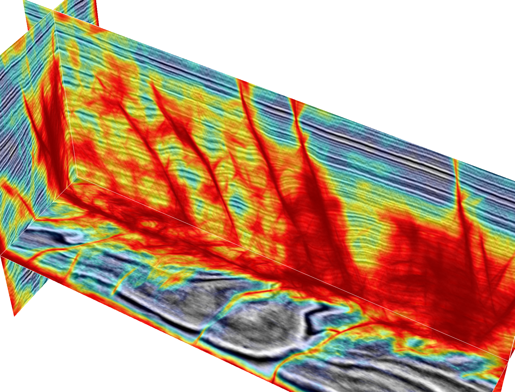
Automatic fault interpretation with optimal surface voting
This work will be presented at the 2018 SEG annual meeting:
Presentation Date and Time: October 17, 2018 from 8:30 AM to 8:55 AM
Session Room: 210A (Anaheim Convention Center), in the Anaheim Convention Center
This repository contains computer programs written and used by Xinming Wu for 2D and 3D fault interpretation that is discussed in our Geophysics paper Automatic fault interpretation with optimal surface voting.
If you find this work helpful in your research, please cite:
@article{wu2018automatic,
    author = {Xinming Wu and Sergey Fomel},
    title = {Automatic fault interpretation with optimal surface voting},
    journal = {GEOPHYSICS},
    volume = {83},
    issue = {5},
    pages = {O67-O82},
    year = {2018},
    doi = {10.1190/GEO2018-0115.1},
    URL = {https://library.seg.org/doi/abs/10.1190/geo2018-0115.1},
}
Summary
If you want to do more than browse the source code, you must first download and build the package using Gradle.
Here are brief descriptions of key components:
OptimalSurfaceVoter
Computes optimal voting surfaces, voting scores and a final 3D voting score map.
OptimalPathVoter
Computes optimal voting paths, voting scores and a final 2D voting score map.
FaultOrientScanner2
Quickly scan for approximate fault dips in 2D
FaultOrientScanner3
Quickly scan for approximate fault strikes and dips in 3D
FaultSkinner
Automatically construct fault skins/surfaces from a final voting score map
FaultSkin
A simple linked data structure to represent a fault surface as discussed by Wu and Hale (2016)
Run a demo
-
download the 3D seismic data "xs.dat" into the folder ./data/3d/f3d/
-
go to ./src/osv/ and type ./jy demoF3d.py to run a test on the F3 dataset
Examples
2D and 3D examples published in the paper.
2D examples
1) F3 data in Figures 7 and 8 (provided by the Dutch Government through TNO and dGB Earth Sciences)
Dimensions: n1=380, n2=591
Data type: binary with BIG_ENDIAN
Seismic: ./data/2d/f3d/gx56.dat
Linearity: ./data/2d/f3d/ep56.dat
OSV fault: ./data/2d/f3d/fv.dat
Thinned OSV fault: ./data/2d/f3d/fvt.dat
seismic time/depth slice (left) and 1-planarity (input for optimal path voting)
optimal path voting faults before (left) and after (right) thinning
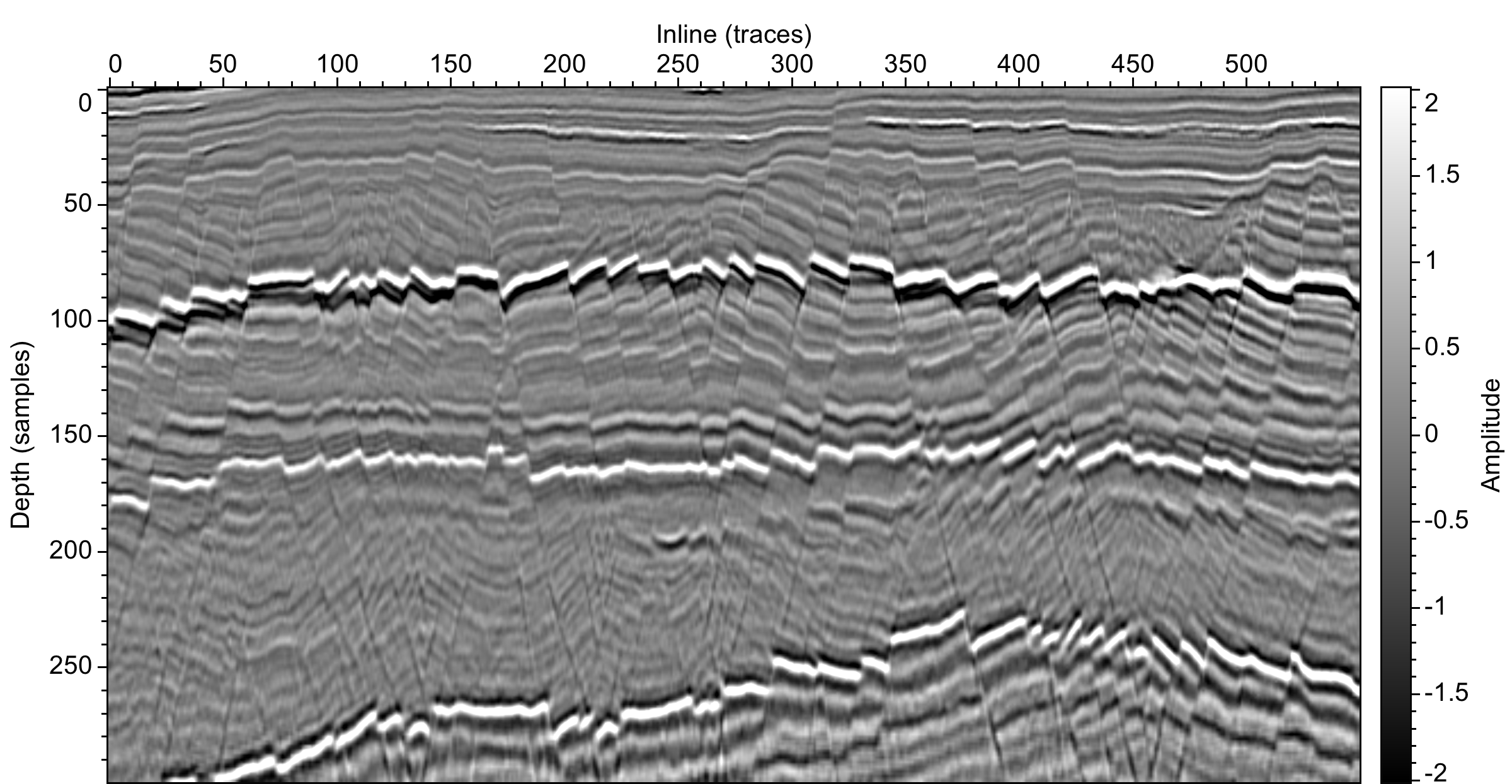
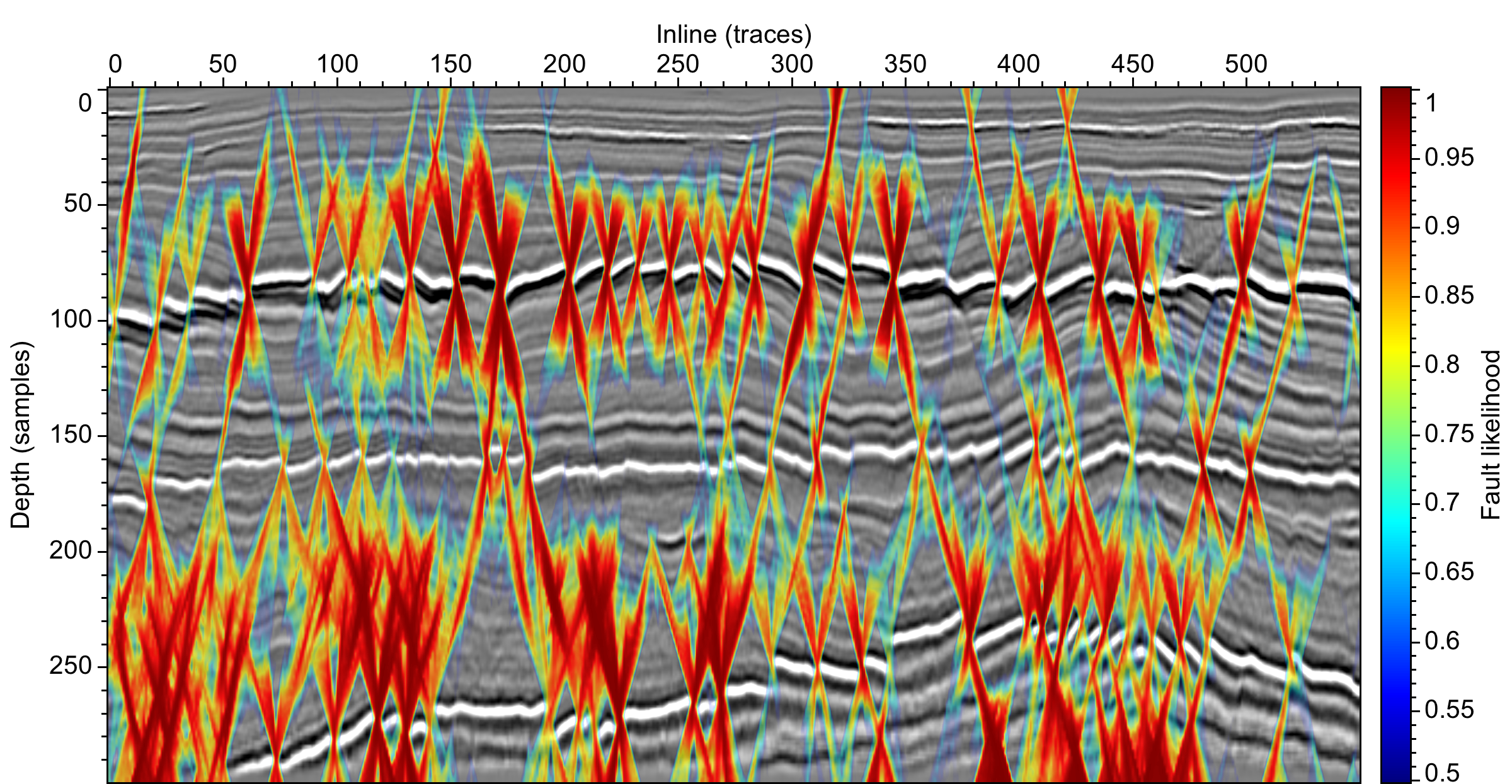
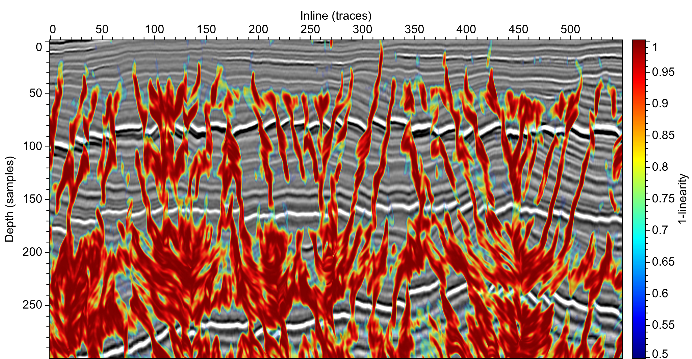
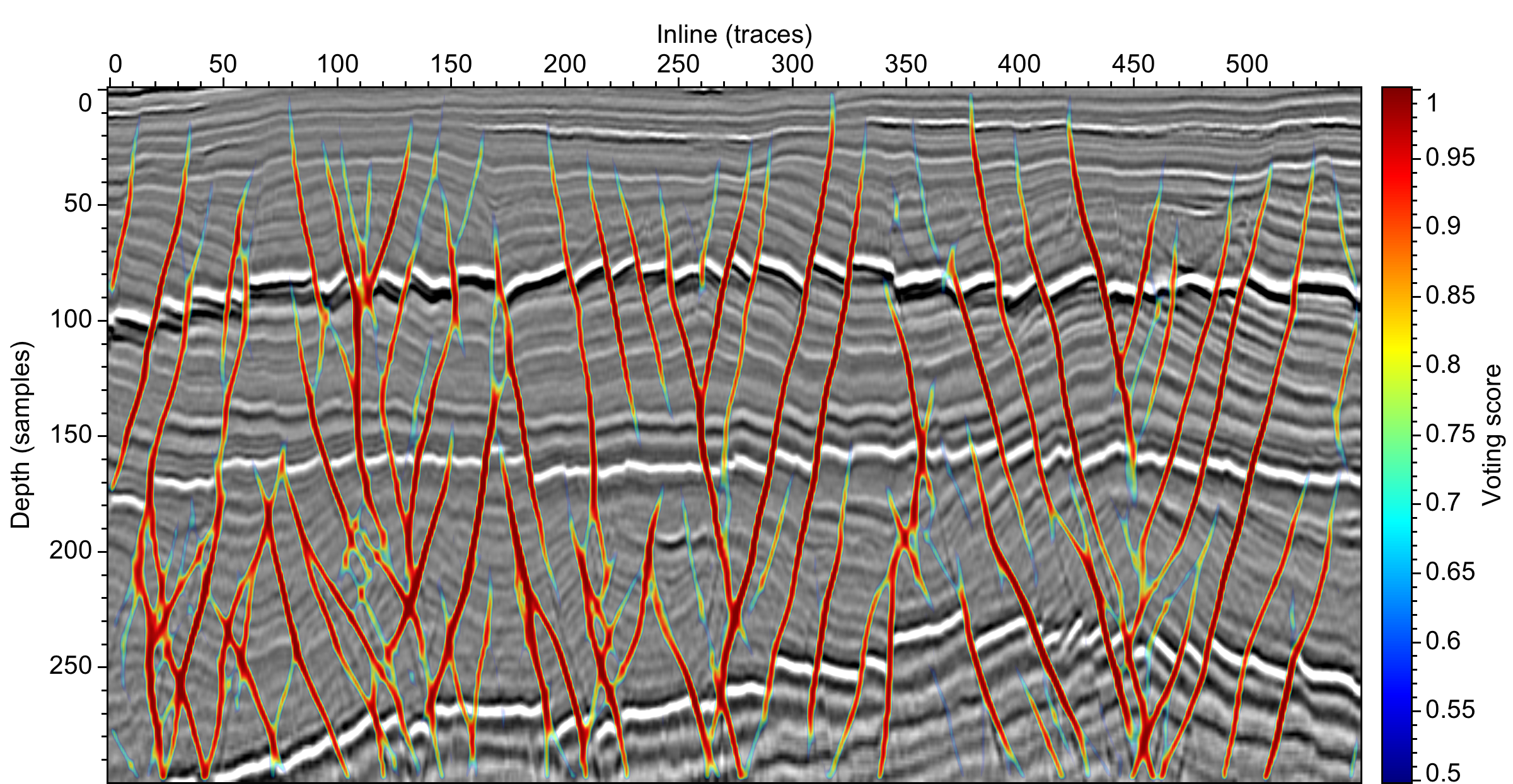
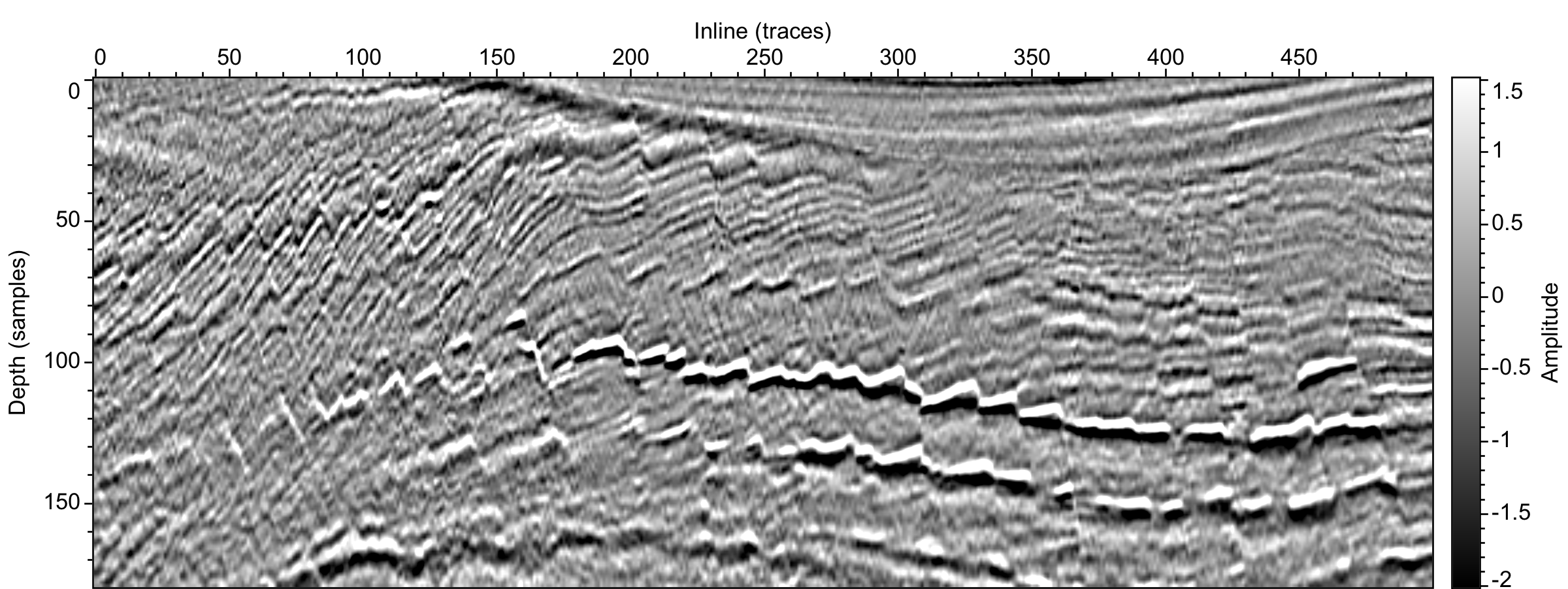
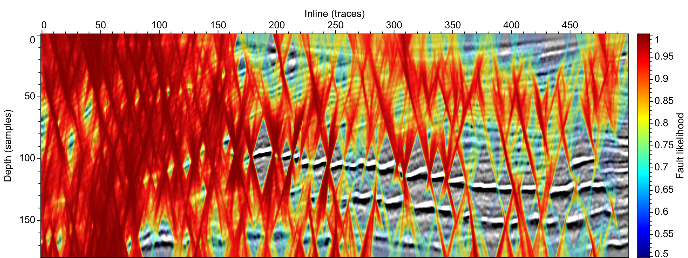
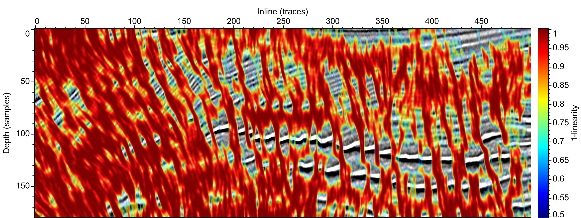
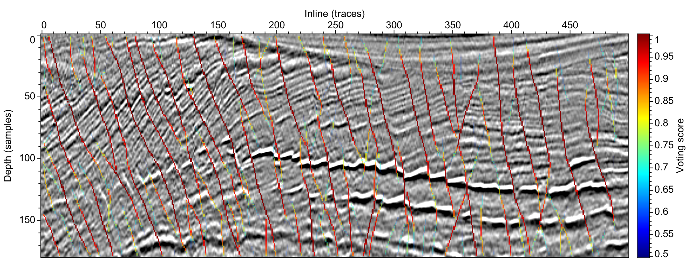
2) Campos data in Figure 9 (seismic data was provided by Dr. Michael Hudec)
Dimensions: n1=300, n2=550
Data type: binary with BIG_ENDIAN
Seismic: ./data/2d/campos/gx373.dat
OSV fault: ./data/2d/campos/fv.dat
Thinned OSV fault: ./data/2d/campos/fvt.dat
---------------------seismic image (left) and fault likelihood (Hale, 2013; Wu and Hale, 2016)-----------------------
input 1-linearity (left) and output optimal path voting faults (right)
3) Costa Rica data in Figure 10 (acquired in the subduction zone, Costa Rica Margin, provided by Dr. Nathan Bangs)
Dimensions: n1=210, n2=825
Data type: binary with BIG_ENDIAN
Seismic: ./data/2d/crf/gx3366.dat
OSV fault: ./data/2d/crf/fv.dat
Thinned OSV fault: ./data/2d/crf/fvt.dat
Fault likelihood: ./data/2d/crf/fl.dat
Thinned fault likelihood: ./data/2d/crf/flt.dat
---------------------seismic image (left) and fault likelihood (Hale, 2013; Wu and Hale, 2016)-----------------------
input 1-linearity (left) and output optimal path voting faults (right)
3D examples
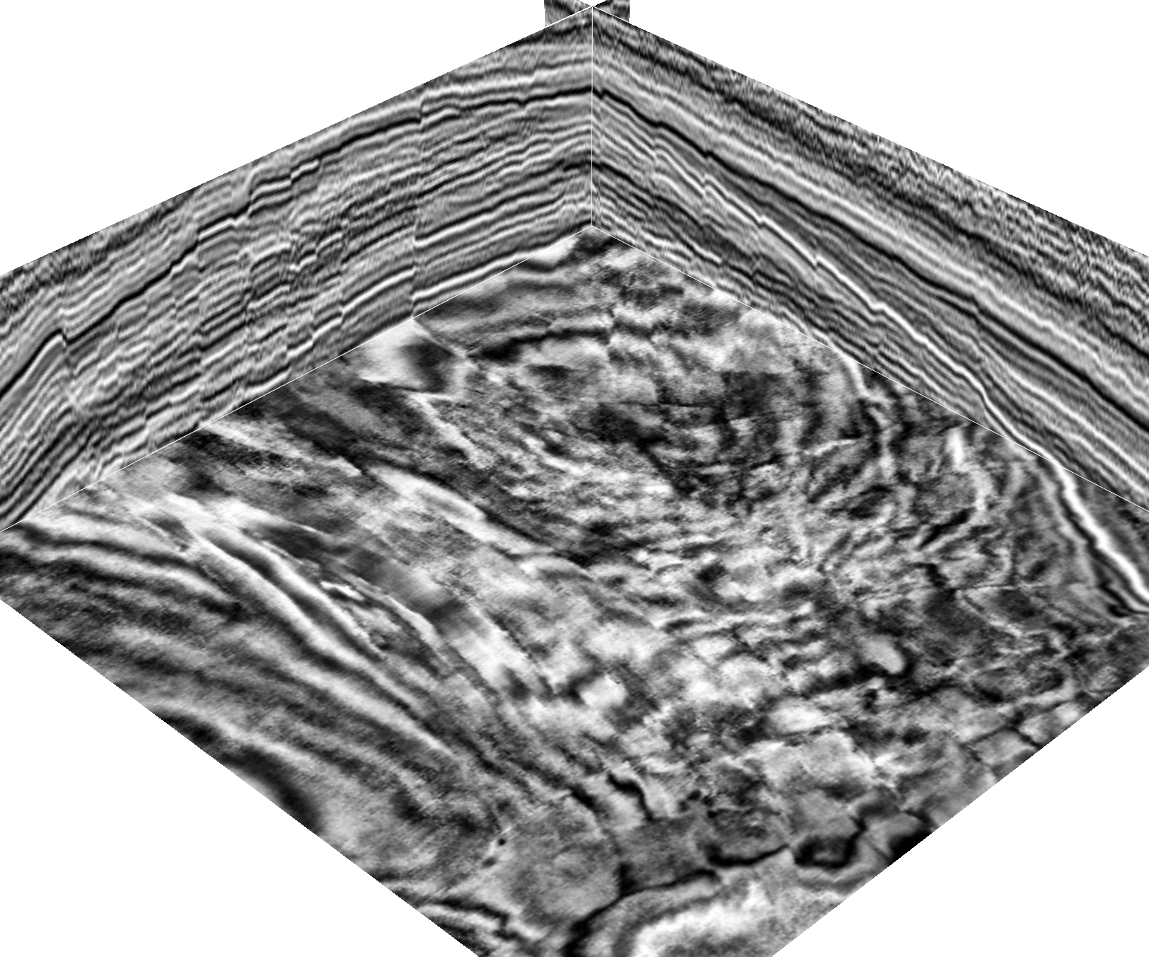
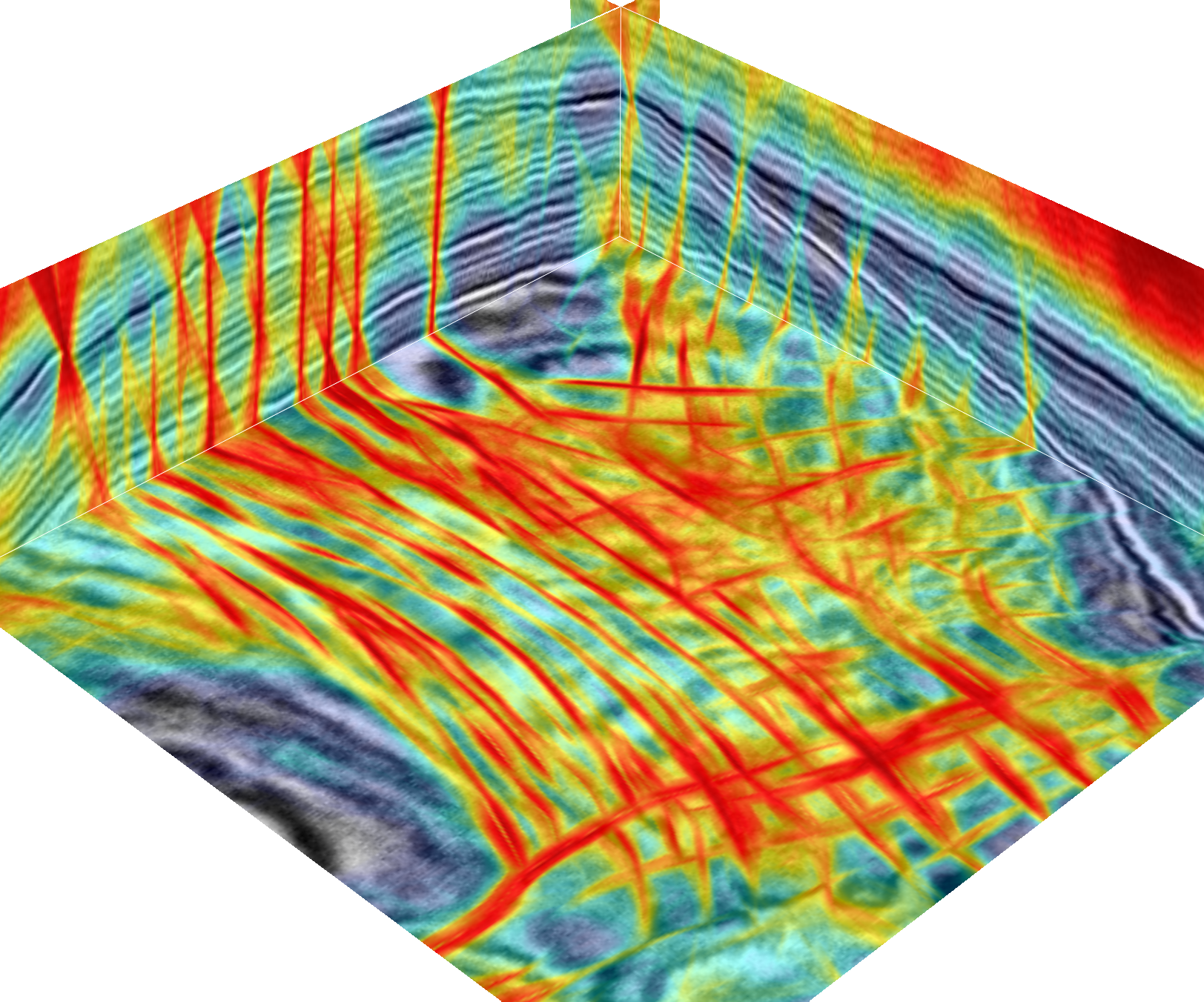
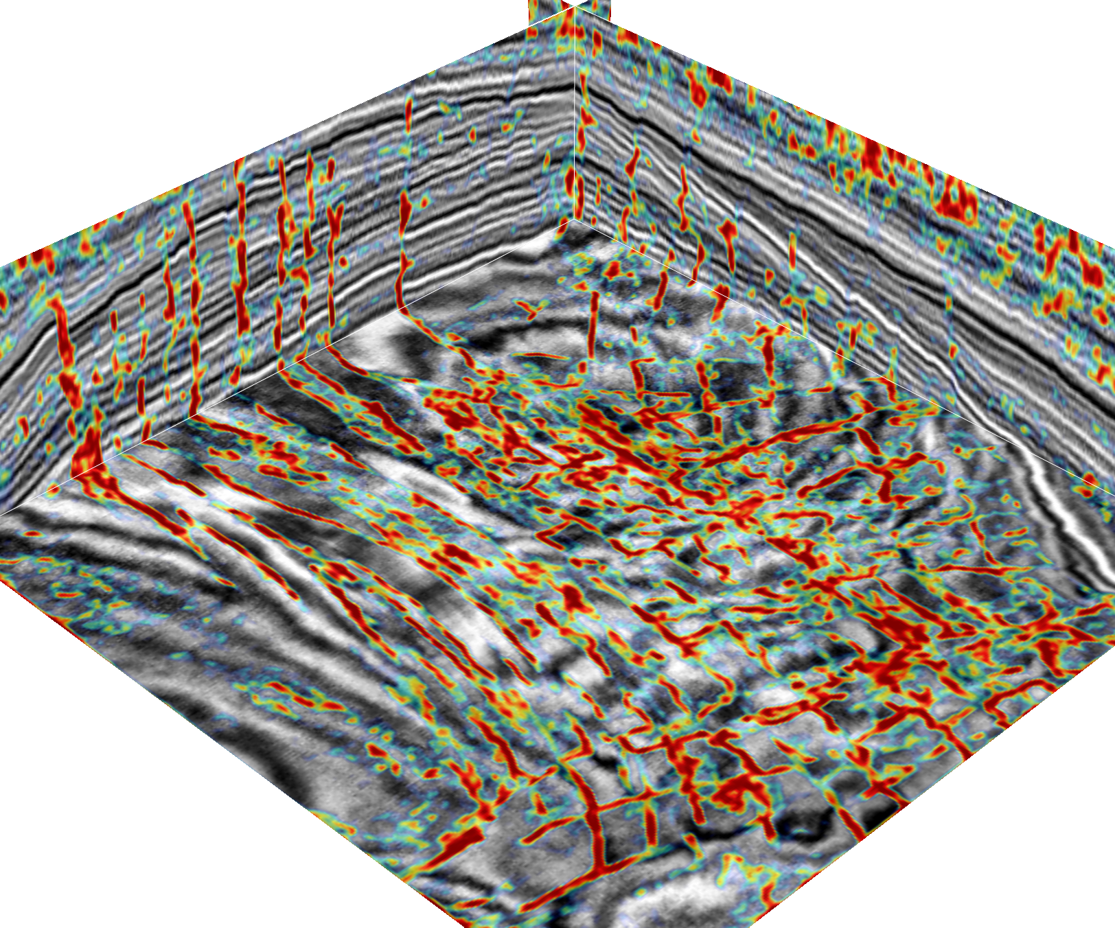
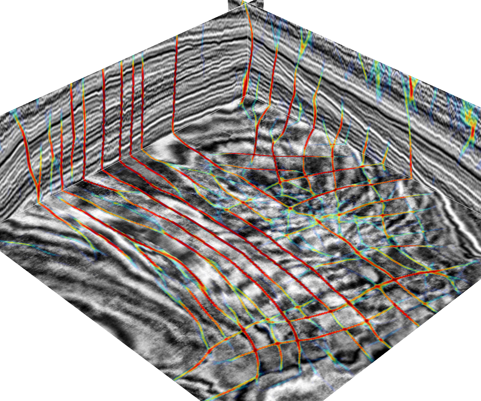
1) F3 data in Figure 11 (provided by the Dutch Government through TNO and dGB Earth Sciences)
The datasets can be downloaded from: https://drive.google.com/open?id=1InfMvCSZWdJclykiTBIXDgV7HYdBj5_K
Dimensions: n1=100, n2=400, n3=420;
Data type:binary with BIG_ENDIAN
Seismic: xs.dat;
Input planarity: ep.dat
Output OSV fault: fv.dat
Thinned OSV fault: fvt.dat
Fault likelihood: fl.dat
---------------------seismic image (left) and fault likelihood (Hale, 2013; Wu and Hale, 2016)-----------------------
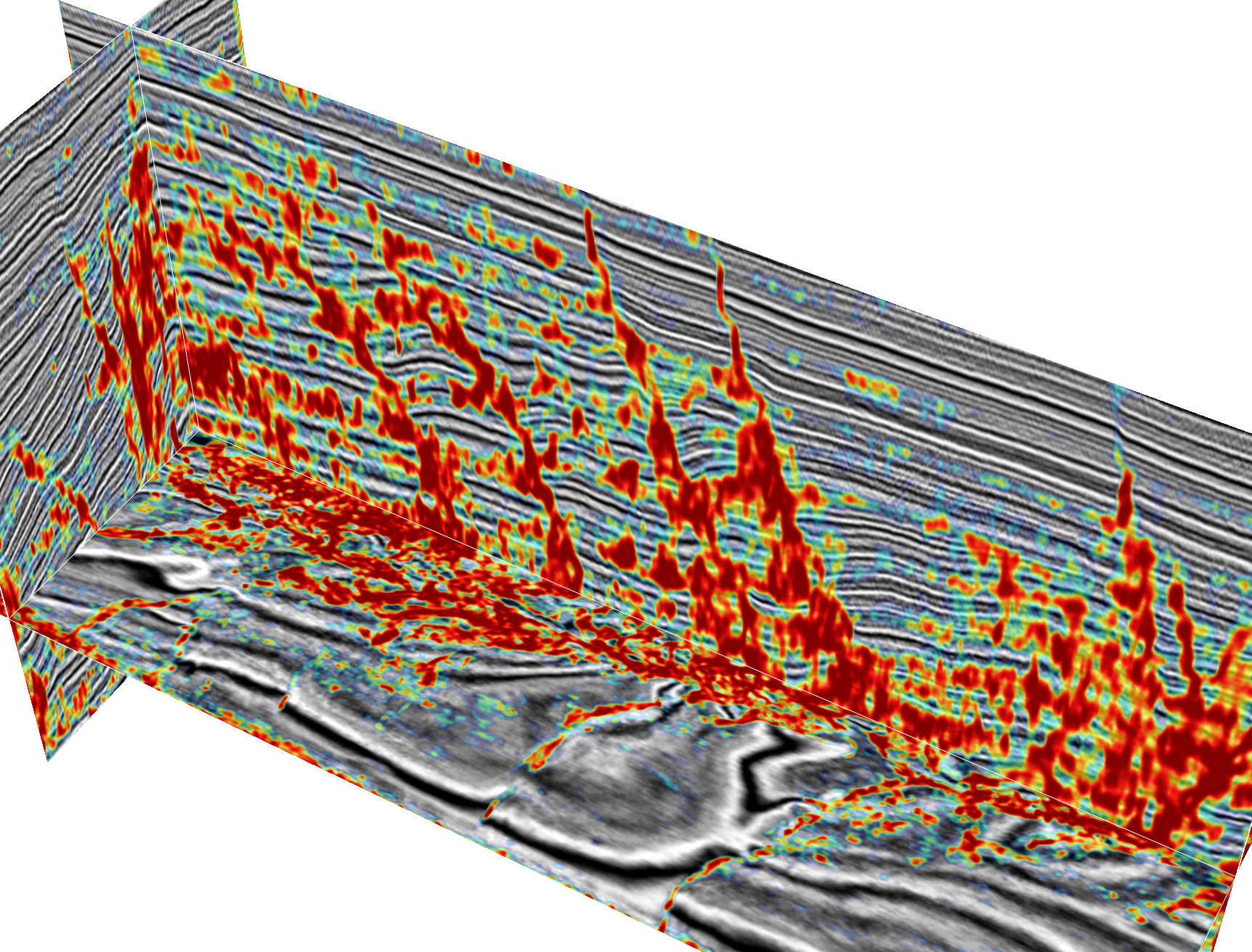
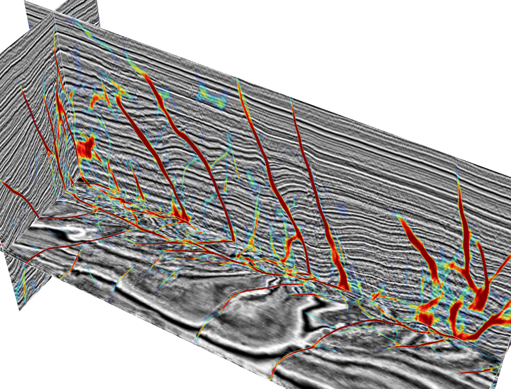
input 1-planarity (left) and output optimal surface voting (OSV) fault (right)
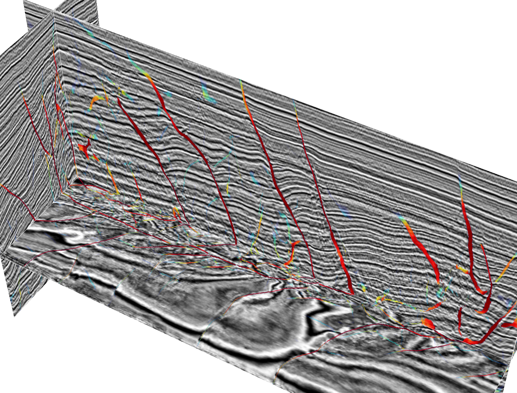
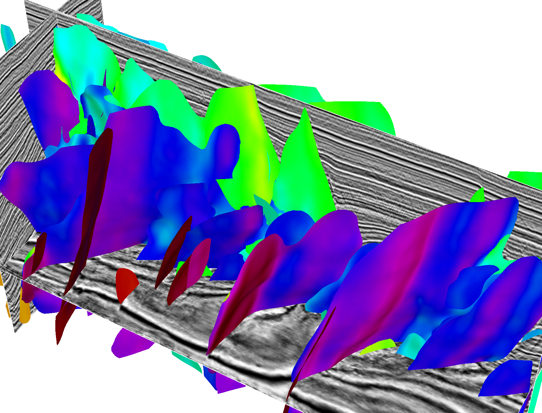
thinned OSV fault (left) and automatic fault surfaces colored by fault strike (right)
2) Clyde data in Figures 14 and 15 (provided by Clyde through Paradigm)
The datasets can be downloaded from: https://drive.google.com/open?id=10x1uO-GBJekmD2wS7S6VFbVsrxGXzMCC
Dimensions: n1=400, n2=801, n3=300
Data type:binary with BIG_ENDIAN
Seismic: gx.dat
OSV fault: fv.dat
---------------------seismic image (left) and fault likelihood (Hale, 2013; Wu and Hale, 2016)-----------------------
input 1-planarity (left) and output OSV fault (right)
thinned OSV fault (left) and automatic fault surfaces colored by fault strike (right)
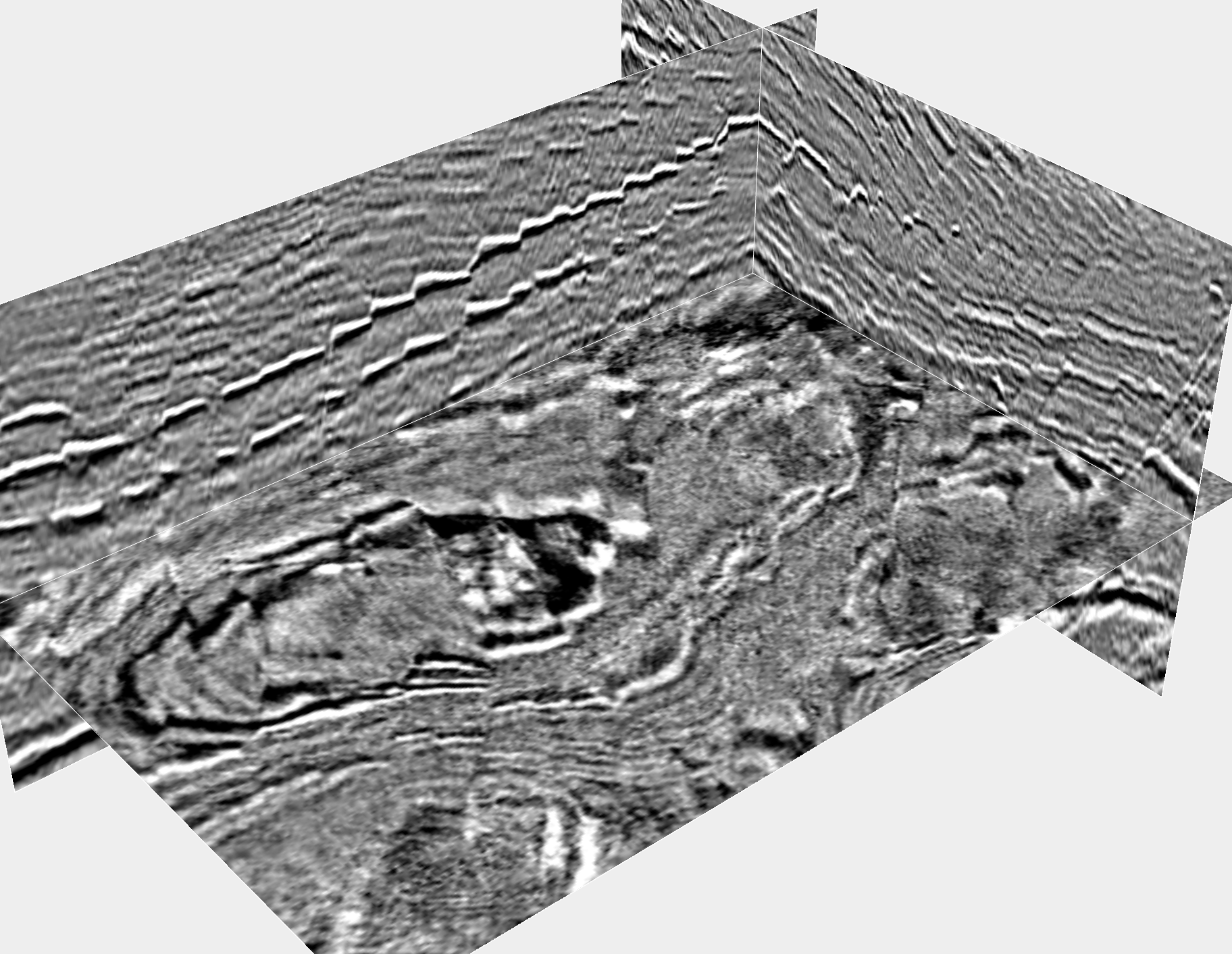
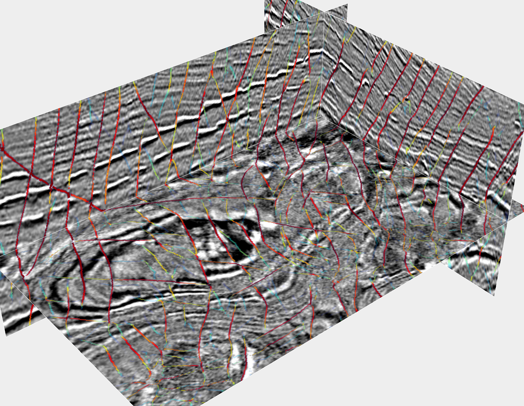
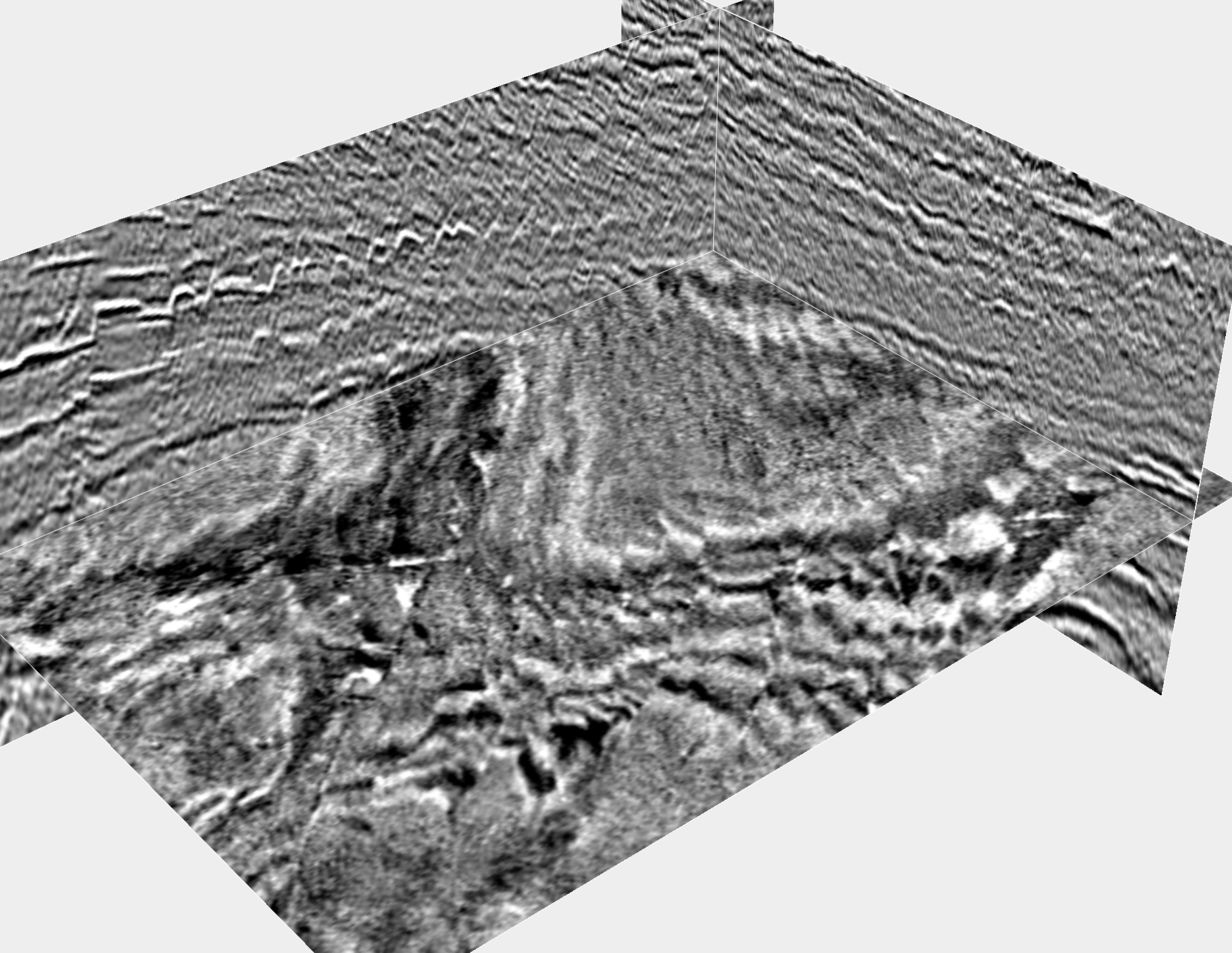
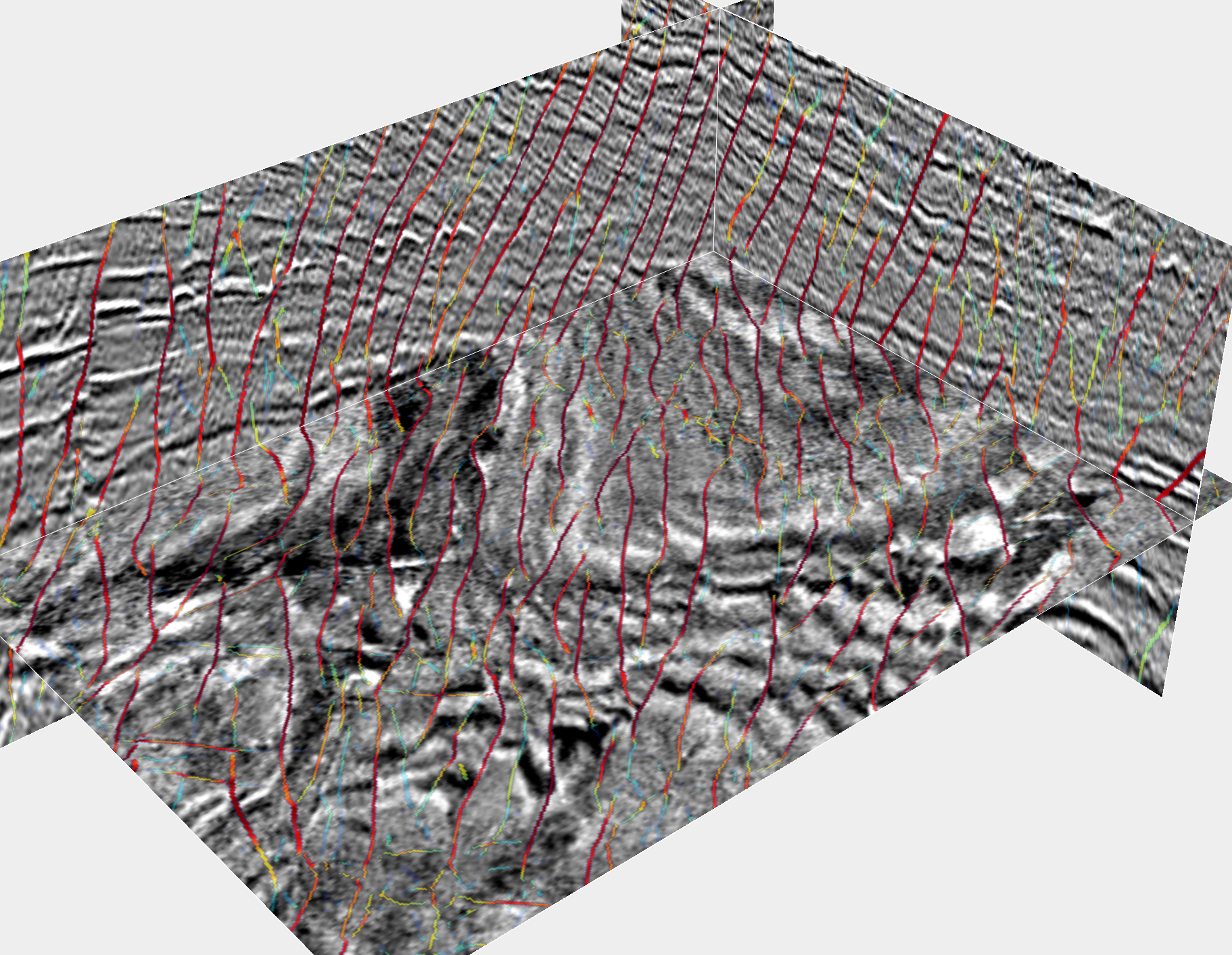
3) Costa Rica data in Figure 16 (acquired in the subduction zone, Costa Rica Margin, provided by Nathan Bangs)
The datasets can be downloaded from: https://drive.google.com/open?id=1fjZuonXYc55ytiKiFboUVkQWVRbht0yQ
Dimensions: n1=210, n2=920, n3=825;
Data type:binary with BIG_ENDIAN
Seismic: gx.dat;
OSV fault: fv.dat;
Thinned OSV fault: fvt.dat;
seismic image (left) and thinned OSV fault (right)
seismic image (left) and thinned OSV fault (right)
Copyright (c) 2018, Xinming Wu. All rights reserved. This software and accompanying materials are made available under the terms of the Common Public License - v1.0, which accompanies this distribution.
