Notification

Hi there, thanks for exploring this repository. It has currently been archived. Please refer to here.

Numerical Optimization

People optimize. This is a repo for my notes and exercise of Book Numerical Optimization by J. Nocedal, S.J. Wright

Chapter 1 Introduction

⭐Elements of optimization📦

objective: sth. need to be first defined with quantitative measure.

variable / unknown: the characteristics of the system, which can optimize the objective

constraint : the constraint of variables

modeling : the process identifying objectives, variables, and constraints for a given problem

algorithm : no universal one, but should find the tailored one related to the objective

optimality condition : mathematical expression checking whether it is a good solution

sensitivity analysis : possible solution to improve

1.1 Mathematical Formulation

⭐(mathematical speaking) Optimization is the minimization / maximization of a function subject to constraints on its variables.

$x$ - variable, unknown, parameters(vector向量)
$f$ - objective function目标函数(scalar function) of $x$
$c_i$ - constraint function约束函数(scalar function) of $x$ where must be satisfied
$\Omega$ - feasible domain可行域

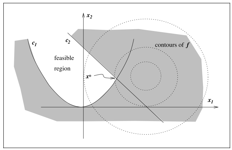
$$ \min_{x\in\R^n}\space f(x)\space\space\text{subject to}\space\space \begin{cases} c_i(x)=0, & i\in\Epsilon \text{, Equality等式}\\ c_i(x)\geq0, & i\in I\text{, Inequality不等式} \end{cases}\\ \Omega = {x: C_i(x)=0, i\in\Epsilon,C_i(x)\geq0,i\in\ I } $$

Let's take an example: $$ \min(x_1-2)^2+(x_2-1)^2\space\space \text{subject to} \begin{cases} x_1^2-x_2\leq0, \ x_1+x_2\leq2. \end{cases} $$ $(x_1-2)^2+(x_2-1)^2$ is a bunch of contour(等值线)

$x_1^2-x_2\leq0$ is parabolic curve

$ x_1+x_2\leq2$ is a linear curve

The above equation can be illustrated as followed:

The above equations can be written as followed: $$ f(x) =(x_1-2)^2+(x_2-1)^2, \quad x=\begin{bmatrix}x1\x2\end{bmatrix},\ c(x)=\begin{bmatrix}\quad c_1(x)\quad\\quad c_2(x)\quad\end{bmatrix}=\begin{bmatrix}-{x_1}^2+x_2\\quad-x_1+-x_2+2\quad\end{bmatrix}, I={1,2}, E=\empty $$ :heavy_check_mark: The $x^*$ is the minimal solution.

1.2 A Transportation Problem

$F_i$ : factory

$a_i$: tons of certain products by factory $F_i$

$R_i$: Retail outlets

$b_i$: demands of tons of the product by retail outlet $R_i$

$c_{ij}$: cost of shipping per ton of the product from $F_i$ to

$x_{ij}, i=1,2, j=1,...,12$: where $x_{ij}$ is the number of tons of product shipped from factory $F_i$ to retail outlet $R_j$

To conclude, the optimization can be written as:

$$ \begin{aligned} \text{min}&\sum_{ij}c_{ij}x_{ij}\\ \text{subject to }&\sum_{j=1}^{12}x_{ij}\leq a_i,\quad i=1,2\\ &\sum_{i=1}^{2}x_{ij}\geq b_j,\quad j=1,...,12\\ &x_{ij}\geq0,\quad i=1,2, \quad j=1,...,12 \end{aligned} $$

⭐This is a linear problem.

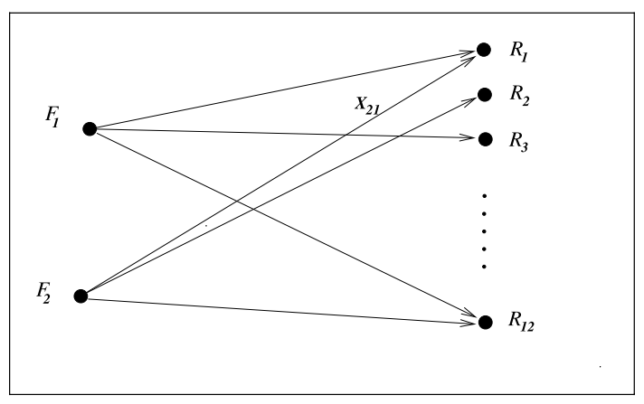
But if there is a fee for storing product, then the cost is $$ \sum_{ij}c_{ij}\sqrt{{\epsilon}+x_{ij}} $$ :star: This is a non-linear problem!

1.3 Continuous Versus Discrete Optimization

📌 Difficulty: continuous optimization < discrete optimization.

continuous optimization:

$x$ is infinite, real number

example in 1.1

discrete optimization:

$x$ is finite, the output may be changed significantly as we vary $x$

integer programming : constraints, which have the form $x_i ∈ Z$,where $Z$ is the set of integers($x_i ∈{1,2,5}$), or binary constraints($x_i ∈{0, 1}$)

mixed integer programming(MIP) : both integer or binary constraints.

1.4 Constrained and Unconstrained Optimization Problems

📌 Difficulty: unconstrained optimization无约束优化 < constrained optimization约束优化

Unconstrained optimization

e.g. $E = I = \empty$

Constrained optimization

e.g. $0\leq x_i\leq 100,\sum_ix_i\leq1$

1.5 Global and Local Optimization

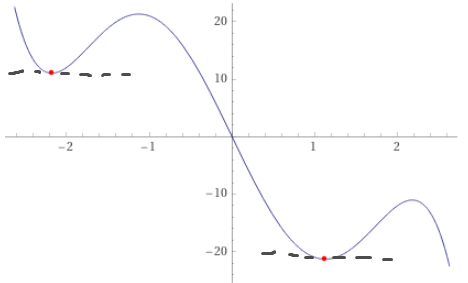
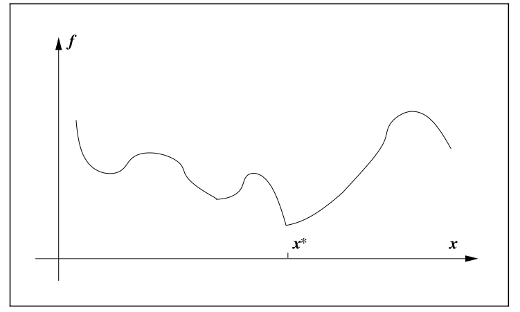
📌 Difficulty: local optimization < global optimization

In linear programming / convex programming:

global solution = local solution

In non-linear programming:

tend to find local solution, since global is hard to find

1.6 Stochastic and Deterministic Optimization

Certainty:

Deterministic optimization

Uncertainty:

stochastic optimization => a number of possible scenarios to optimize the expected performance

chance-constrained optimization => ensure $x$ satisfy constraints with some probability

robust optimization => certain constraints to hold for all possible values of the uncertain data.

1.7Convexity

⭐This is the fundamental concept in optimization. In CHN, convex is 凸，not 秃

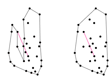
Convex Set Definition: A set $S \in \mathbb{R}^n$ is a convex set if line connecting any two points lies inside $S$. For any two points $x\in S\space\text{and}\space y\in S$, we have $ax+(1-a)y\in S$ , for all $a\in [0,1]$

Left: Non-convex, Right: Convex

Convex Function: its domain 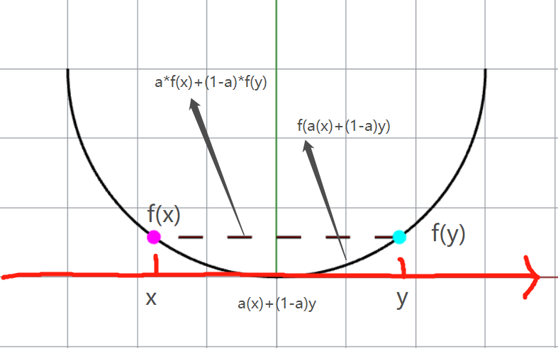$S$ is a convex set and for any two point $x$ and $y$ in $S$, the following is satisfied: $$ f(ax+(1-a)y)\leq af(x)+(1-a)f(y), \quad \text{for all }a\in [0,1] $$

❓ You may wonder is this convex?? why not concave?? Yes, function is said to be concave if it is convex.

Strictly convex: $x\neq y$ in the formula (6) AND $a$ is in the open interval $(0,1)$

Linear function = convex: $$ f(x)=c^Tx+a $$

$c$ : vector $\in\mathbb{R}$

$a$: scalar

Quadratic function = convex: $$ f(x) = x^T Hx $$

$H$ : symmetric positive semidefinite matrix

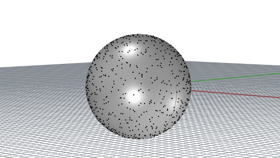
Unit ball = convex: $$ {y ∈ \mathbb{R}^n\quad |\quad\norm{y}_2\leq 1} $$

polyhedron = convex: $$ {x ∈ \mathbb{R}^n\quad |\quad Ax = b, \quad Cx ≤ d} $$

$A,C$: matrices of appropriate dimension

$b, d$ :vectors.

⭐ If the objective function in the optimization problem (formula 1) and the feasible region are both convex, then any local solution of the problem is in fact a global solution.

Convex programming

It is a special case of general constrained optimization problem.

the objective function is convex,

the equality constraint functions $c_i (·), i ∈ E, $are linear

the inequality constraint functions $c_i (·), i ∈ I$,are concave.

1.8Optimization Algorithms

⭐ They are all iterative process.

Good algorithms must:

Robustness, Efficiency, Accuracy

The wisdom is to manage the tradeoffs between convergence rate and storage requirements, and between robustness and speed, and so on, are central issues in numerical optimization. Because no algorithm is perfect and they all have pros and cons.

Chapter 2 Fundamentals of Unconstrained Optimization

Unconstrained Optimization：

1. variable: real number$\mathbb{R}$ with no restrictions(infinite)

2. formula: $\text{min}_xf(x)$

3. $x\in \mathbb{R}^n$ : is a real vector, $n\geq 1$

4. $f:\mathbb{R}^n \to \mathbb{R}$ , is a smooth function

5. characteristic:lack of global perspective on the function(due to 1.), only some scope on $x_1,x_2,...$

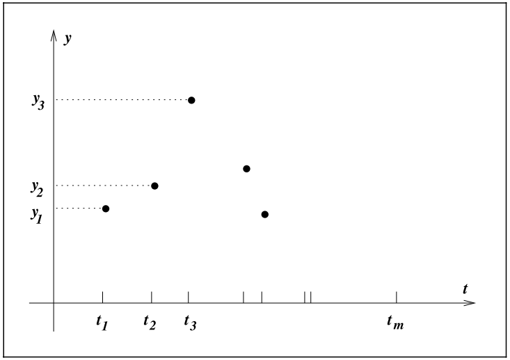
Example on unconstrained optimization:

Least squares data fitting problem Taking the above problem, we can take down the process into

inspect the data

deduce the signal with possible solution

detect exponential and oscillatory behavior

write a formula

$\phi(t;x)=x_1+x_2e^{-(x_3-t^2)/4}+x_5cos(x_6t)$

$t$: times at $x$ axis, (input)

y: output

$x_i,i=1,2,...6$ : the parameter of the model

therefore $x_i$ can also be written as a vector: $x=(x_1,x_2,...,x_6)^T$

What to do? Minimize the discrepancy between $\phi(t;x)$ and $y_t$

$r_j(x)=y_j-\phi(t_j;x),\quad j=1,2,...,m$ m is the amount of input data

Written formally: $$ \min_{x\in\mathbb{R}^6} f(x)=r_1^2(x)+r_2^2(x)+...+r_m^2(x) $$ :star:This is so-called non-linear least-squares problems(非线性最小二乘问题).

Quick question why square the $r_i$? Because the residual can be negative.

2.1What is a solution?

Global minimizer:

A point $x^$ is a global minimizer if $f(x^)\leq f(x)$ for all $x\in\mathbb{R}^n$

Local minimizer:

A point $x^∗$ is a local minimizer if there is a neighborhood $N$ of $x^∗$ such that $f(x^∗) ≤ f(x)$for all $x ∈ N$.

Weak local minimizer:

copy definition from local minimizer, + when $N$ is an open set that contains $x^$ , e.g. $N=[0,2], x^=2$

e.g. $f(x)=2$, where every point is weal local minimizer

Strict/Strong local minimizer:

A point $x^∗$ is a strict local minimizer if there is a neighborhood $N$ of $x^∗$ such that $f(x^∗) < f(x)$for all $x ∈ N$ with $x\neq x^*$.
e.g. f(x)=(x-2)^2

Isolated local minimizer:

This is a little bit confusing thinking together with strict local minimizer.

:star: The solid conclusion is isolated local minimizer $\subset$ strict local minimizer

What the hell?! OK, please recall the methodology of infinity and look at the following formula:

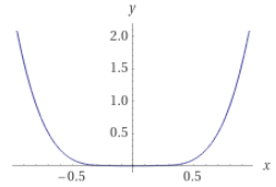
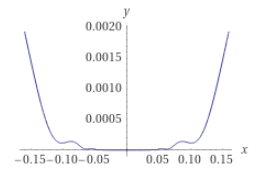
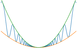
$f(x)=x^4cos(1/x)+2x^4$

Nothing special in the beginning, but if we zoom in around 0, we can notice that the curve oscillates very much!! Therefore, if we think about $x_j\to0$, there are infinite points are local minimizer whose value=0. Therefore $j\to\infin$, there are many many strict local minimizers but NONE of them are isolated local minimizer.

So in future practice, we should pay attention to those crazy function may be "trapped".

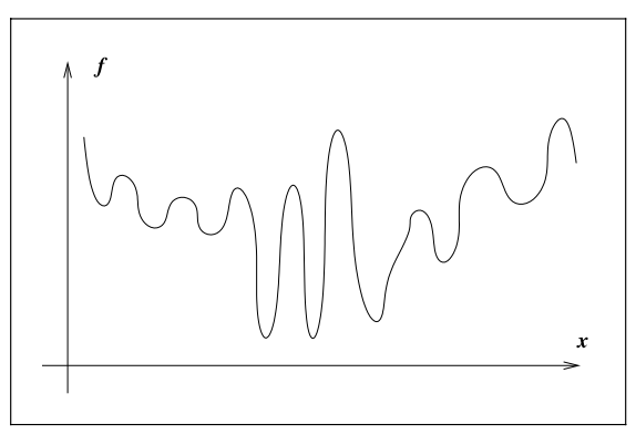
A difficult case for global minimization

Recognizing a local minimum

How to recognize a local minimum without examining all the points?

:star:In particular, if $f$ is twice continuously differentiable, we may be able to tell that $x^∗$ is a local minimizer (and possibly a strict local minimizer) by examining just the gradient $∇ f(x^∗)$ and the Hessian $∇^2 f(x^∗)$.

In the following, few theorem will be used and introduced multiple times.

Theorem 2.1 (Taylor's Theorem)

Prerequisites: $f :\mathbb{R}^n → \mathbb{R}$ is continuously differentiable and that $p ∈ \mathbb{R}^n$ (first continuously differentiable)

then we have:

$$ f(x + p) = f(x) +∇ f(x + tp)^T p, $$

for some $t\in (0,1)$, if $f$ is twice continuously differentiable,

then we have:

$$ ∇ f(x + p) =∇ f(x) +\int^{1}_{0}∇^2 f(x + tp)pdt\\ f(x + p) = f(x) +∇ f(x)^T p + \frac{1}{2} p^T∇^2 f(x + tp)p $$

Theorem 2.2 (First-Order Necessary Conditions)

Prerequisites: If $x^∗$ is a local minimizer and $f$ is continuously differentiable in an open neighborhood of $x^∗$,

then we have:

$$ ∇ f(x^∗) = 0 $$

To see it geometrically:

Fun fact: the point $x^*$ are also called stationary point.

// TODO Explain and proof

Theorem 2.3 (Second-Order Necessary Conditions)

Prerequisites: $x^∗$ is a local minimizer of $f$ and $∇^2 f$ exists and is continuous in an open neighborhood of $x^*$,

then we have:

$$ ∇ f(x^∗) = 0 \text{ and }∇^2 f(x^∗) \text{ is positive semidefinite} $$

// TODO Explain and proof, and add texts of positive semidefinite.

Theorem 2.4 (Second-Order Sufficient Conditions)

Prerequisites: $∇^2 f$ is continuous in an open neighborhood of $x^∗$ and that $∇ f(x^∗)= 0$ and $∇^2 f(x^∗)$ is positive definite,

then we have:

$$ x^∗ \text{ is a strict local minimizer of }f $$

// TODO add example and proof

Theorem 2.5

Prerequisites: When $f$ is convex, then we have:

$$ \text{any local minimizer }x^∗ \text{ is a global minimizer of }f $$

Prerequisites: if in addition $f$ is differentiable, then we have:

$$ \text{any stationary point } x^∗\text{ is a global minimizer of }f $$

Conclusion of theorem 2.1 to 2.5

These results, which are based on elementary calculus, provide the foundations for unconstrained optimization algorithms. In one way or another, all algorithms seek a point where $∇ f(·)$ vanishes.

Non-smooth Problem

What it is?

Geometrically, the nonsmooth function consists of a few smooth pieces, with discontinuities between the pieces.

So what we gonna do?

It may be possible to find the minimizer by minimizing each smooth piece individually, a.k.a. examing the subgradient and generalized gradient.

(a side note, this book will not cover non-smooth problem.)

2.2Overview of algorithm

All algorithms for unconstrained minimization require the user to supply a starting point, which we usually denote by $x_0$

XingxinHE / NumericalOptimization