MathFor3DAndCG

Study notes of Mathematics for Lengyel, Eric. 3D Game Programming and Computer Graphics. 2011

Notation Convention

Quantity/Operation	Notation/Examples
Scalars	Italic letters: $x,t,A,a,\omega$
Angles	Italic Greek letters: $\theta,\phi,a$
Vectors	Boldface letters: $\bold{V, P, x, \omega}$
Quaternions	Boldface letters: $\bold{q_1, q , q_2}$
Matrices	Boldface letters: $\bold{M,P}$

Quick Reference

2. Vector

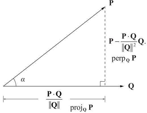
📌Dot Products The dot product between two $n$-dimensional vectors $P$ and $Q$ is a scalar defined by $$ P\cdot Q=\sum_{i=1}^{n}P_iQ_i=P_1\cdot Q_1+P_2\cdot Q_2+...+P_n\cdot Q_n $$ The dot product is related to the angle $a$ between the vectors $P$ and $Q$ by the formula $$ P\cdot Q = \norm{P}\norm{Q}\cos{a} $$

📌Vector Projections

The projection of a vector $P$ onto a vector $Q$ is given by $$ \text{proj}_QP = \frac{P\cdot Q}{\norm{Q}^2}Q $$ and the component of $P$ that is perpendicular to $Q$ is given by $$ \text{perp}_QP &= P-\text{proj}_QP\ &=P-\frac{P\cdot Q}{\norm{Q}^2}Q $$

📌Cross Products

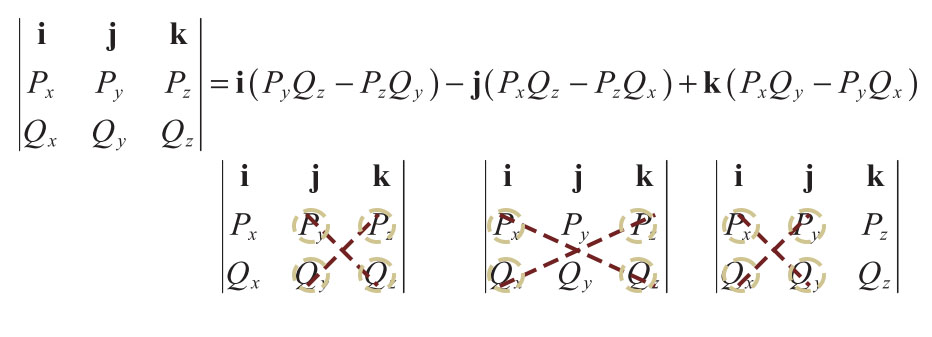
The cross product between two 3D vectors $P$ and $Q $is a 3D vector defined by $$ P\cross Q = \langle P_yQ_z-P_zQ_y,\space P_zQ_x-P_xQ_z,\space P_xQ_y-P_yQ_x\rangle $$ This can also be written as the matrix-vector product $$ P\cross Q= \begin{bmatrix} 0&-P_z&P_y\ P_z&0&-P_x\ -P_y&P_x&0 \end{bmatrix} \begin{bmatrix} Q_x\Q_y\Q_z \end{bmatrix} $$ The magnitude of the cross product is related to the angle $a$ between the vectors $P$ and $Q$ by the formula $$ \norm{P\cross Q}=\norm{P}\norm{Q}\sin{a} $$

📌Gram-Schmidt Orthogonalization

A basis $\Beta={e_1,e_2,...,e_n}$ for an $n$-dimensional vector space can be orthogonalized by constructing a new set of vectors $\Beta'={e_1',e_2',...,e_n'}$ using the formula $$ e_i'=e_i-\sum_{k=1}^{i-1}\frac{e_i\cdot e_k'}{e_k'^2}e_k' $$

3. Matrices

📌 Matrix Products

If there are matrices $F$($n\cross m_1$) and $G(m_2\cross p)$, the prerequisite for a valid matrix multiplication is that $m_1=m_2$. Then the product is a matrix with shape $n\cross p$. The $i,j$ element of the matrix is: $$ (FG){ij} = \sum{k=1}^{m}F_{ik}G_{kj} $$

📌 Determinants

The determinant of an $n\cross n$ matrix $M$ is given by the formulas

the $cofactor C_{ij}(M)$ of the matrix entry $M_{ij}$ a $$ \begin{align} \text{det}M =& \sum^{n}{i=1}M{ik}C_{ik}(M)\

\text{and}\

\text{det}M =& \sum^{n}{j=1}M{kj}C_{kj}(M)\\

\text{where }C_{ij}(M)\text{ is the cofactor of }M_{ij}\text{defined by}\ C_{ij}(M)\equiv(-1)^{i+j}\text{det}M^{{i,j}}\\\

\text{Example of determinant of 22 and 33 matrix}\\

\text{ det}\bigg(\begin{bmatrix}a&b\c&d\end{bmatrix}\bigg) =& ad-bc

\text{det} \Bigg( \begin{bmatrix} a&b&c\ d&e&f\ g&h&i \end{bmatrix} \Bigg) =&a\text{ det}\bigg(\begin{bmatrix}e&f\h&i\end{bmatrix}\bigg)\ -&b\text{ det}\bigg(\begin{bmatrix}d&f\g&i\end{bmatrix}\bigg)\ +&c\text{ det}\bigg(\begin{bmatrix}d&e\g&h\end{bmatrix}\bigg)\ \end{align} $$

📌 Matrix Inverse

An $n\cross n$ matrix $M$ is invertible if and only if the columns of $M$ form a linearly independent set. Equivalently, $M$ is invertible if and only if $\text{det}M≠0$ .

The entries of the inverse $G$ of an $n\cross n$ matrix $F$ can be calculated by using the explicit formula $$ G_{ij} = \frac{C_{ji}(F)}{\text{det}F} $$ Therefore, a $2\cross 2$ matrix $A$ is given by $$ A^{-1}=\frac{1}{\text{det}A}\begin{bmatrix}A_{22}&-A_{12}\-A_{21}&A_{11}\end{bmatrix} $$ Notice the negative sign in $A_{12}$ and $A_{21}$. That is because $C_{ij}(M)\equiv(-1)^{i+j}\text{det}M^{{i,j}}$. $1+2$ and $2+1$ are odd, so $(-1)$ is still negative.

📌 Eigenvalues and Eigenvectors

The eigenvalues of an $n\cross n$ matrix $M$ are equal to the roots of the characteristic polynomial given by $$ \text{det}(M-\lambda I) $$ An eigenvector $V$ associated with the eigenvalue $λ$ of the matrix $M$ is given by the solution to the homogeneous linear system $$ (M-λI)V= 0 $$ The eigenvalues of a real symmetric matrix are real, and the eigenvectors corresponding to distinct eigenvalues of a real symmetric matrix are orthogonal.

📌 Diagonalization

If $V_1,V_2,...,V_n$ are linearly independent eigenvectors of an $n\cross n$ matrix $M$, then the matrix $A$ given by $$ A = \begin{bmatrix} V_1&V_2&...&V_n\end{bmatrix} $$ diagonalizes $M$, meaning that $$ A^{−1}MA= \begin{bmatrix} \lambda_1&0&\cdots&0\ 0&\lambda_2&\cdots&0\ \vdots&\vdots&\ddots&\vdots\ 0&0&\cdots&\lambda_n\ \end{bmatrix} $$ where $\lambda_1,\lambda_2,...,\lambda_n$ are the eigenvalues of $M$.

Chapter 2 Vector

2.1 Vector Properties

$n$-dimensional vector $V$:

$$ V = \langle V_1,V_2,...,V_N\rangle $$

vector $V$ (column picture) represented by a matrix with 1 column and $n$ rows:

$$ V = \begin{bmatrix}V_1\V_2\\vdots\V_n\end{bmatrix} $$

vector $V$ (row picture) ,the transpose of their corresponding column vectors:

$$ V^T = [V_1\quad V_2\quad \cdots\quad V_n ] $$

scalar($a$) multiply vector($V$):

$$ aV = Va =\langle aV_1, aV_2,..., aV_n\rangle $$

vector($P$) + vector($Q$): (element-wise operation)

$$ P+Q=\langle P_1+Q_1,P_2+Q_2,..., P_n+Q_n\rangle $$

$\norm{V}$ ,magnitude/norm of an $n$-dimensional vector $V$ is a scalar.

$$ \norm{V} = \sqrt{\sum^{n}_{i=1}{V_i^2}} $$

$\norm{V}$ ,is also the unit length. A vector having a magnitude/ norm is said to be a unit vector.

Taking the 3-dimensional vector as an example,

$$ \norm{V}=\sqrt{V_x^2+V_y^2+V_z^2} $$

vector normalization:

$V$ multiply $\frac{1}{\norm{V}}$

2.2 Dot Product

⭐ Big picture of its application: it measure the difference between the directions in which the two vectors point.

dot product of two vectors, also known as the scalar product or inner product

Definition: The dot product of two $n$-dimensional vectors $P$ and $Q$, is the scalar quantity given by the formula.

$$ P\cdot Q=\sum^{n}_{i=1}P_iQ_i $$

dot product is element-wise operation

$$ P\cdot Q=P_1\cdot Q_1+P_2\cdot Q_2+...+P_n\cdot Q_n $$

dot product represented in matrix format

tips: row vector * column vector = scalar

$$ P^T\cdot Q=[P_1\quad P_2\quad...\quad P_n]\begin{bmatrix}Q_1\Q_2\\vdots\Q_n\end{bmatrix} $$

:pencil: Theorem: Given two $n$-dimensional vectors $P$ and $Q$, the dot product $P\cdot Q$ satisfies the equation. $a$ is the angle between $P$ and $Q$.

$$ P\cdot Q = \norm{P}\norm{Q}\cos{a} $$

:pushpin: Fact: in light of theorem: if two vector $P\cdot Q=0$, they are orthogonal.

:pushpin: Fact: $P\cdot Q>0$, they are on the same side. $P\cdot Q<0$, they are on the opposite side.

:pencil: Theorem: Given any scalar $a$ and any three vectors $P, Q$, and $R$, the following properties hold.

$$ \begin{align} P\cdot Q&= Q\cdot P \\ (aP)\cdot Q&=a(P\cdot Q)\\ P\cdot(Q+R)&= P\cdot Q+ P\cdot R\\ P\cdot P&=\norm{P}^2\\ |P\cdot Q|&\leq \norm{P}\norm{Q} \end{align} $$

:pushpin: Projection: for a vector $P$ projected onto $Q$ can be denoted as

:pushpin:Perpendicular: the projection perpendicular to original vector

$$ \begin{align} \text{proj}_QP &= \frac{P\cdot Q}{\norm{Q}^2}Q\\\ \text{perp}_QP &= P-\text{proj}_QP\\ &=P-\frac{P\cdot Q}{\norm{Q}^2}Q \end{align} $$

2.3 Cross Product

⭐ Big Picture: calculates surface normal at a particular point given two distinct tangent vectors.

cross product is also known as vector product which returns a vector rather than an scalar.

Definition 2.6. The cross product of two 3D vectors $P$ and $Q$, written as $P\cross Q$, is a vector quantity given by the formula

$$ P\cross Q = \langle P_yQ_z-P_zQ_y,\space P_zQ_x-P_xQ_z,\space P_xQ_y-P_yQ_x\rangle $$

cross product in matrix picture(also known as pseudodeterminant), where $i,j,k$ are unit vector:

$$ P\cross Q = \begin{vmatrix} \bold{i}&\bold{j}&\bold{k}\\ P_x&P_y&P_z\\ Q_x&Q_y&Q_z \end{vmatrix}\\\ i=\langle1,0,0\rangle\\ j=\langle0,1,0\rangle\\ k=\langle0,0,1\rangle\\ $$

‼️ Attention: the sign in front of $j$ is negative! Others are positive.

:pencil:Theorem 2.7. Let $P$ and $Q$ be any two 3D vectors. Then:

$$ (P\cross Q)\cdot P=0\(P\cross Q)\cdot Q=0 $$

This is very easy to understand. The dot product between a vector and its orthogonal complement is ZERO because they have nothing aligned.

:pencil: Theorem 2.8. Given two 3D vectors $P$ and $Q$, the cross product $P\cross Q$ satisfies the equation. where $a$ is the planar angle between the lines connecting the origin to the points represented by $P$ and $Q$.

$$ \norm{P\cross Q}=\norm{P}\norm{Q}\sin{a} $$

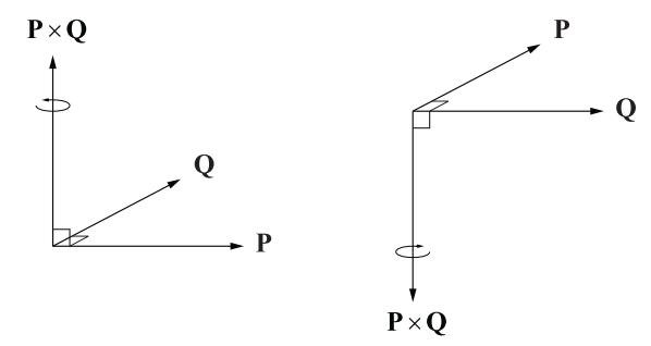
:pushpin:Right hand rule: The cross product is with orientation.

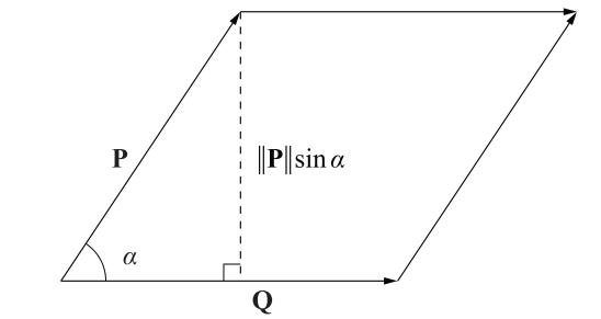
:star: Area of cross product: it is the parallelogram formed by $P$ and $Q$.

$$ \text{Area} = \norm{Q}\cdot\norm{P}\sin{a}=\text{base}\cross\text{height}=P\cross Q $$

:pencil: Theorem 2.9. Given any two scalars $a$ and $b$, and any three 3D vectors $P$, $Q$, and $R$, the following properties hold.

$$ Q\cross P = -(P\cross Q)\\ (aP)\cross Q = a(P\cross Q)\\ P\cross(Q+R)=P\cross Q+P\cross R\\ P\cross P = 0 = \langle0,0,0\rangle\\ (P\cross Q)\cdot R = (R\cross P)\cdot Q = (Q\cross R)\cdot P\\ P\cross(Q\cross P) = P\cross Q\cross P = P^2Q - (P\cdot Q)P $$

:pushpin: Anticommutative, is a characteristic of cross product which implies the order of cross product matters.

$$ (P\cross Q)\cross R \neq P\cross (Q\cross R) $$

2.4 Vector Space

:star: Definition 2.10. A vector space is a set $V$, whose elements are called vectors, for which addition and scalar multiplication are defined, and the following properties hold.

$P\in V,\space Q\in V, \quad \text{s.t. }P+Q\in V$
$P\in V, a\in \mathbb{R}, \text{ s.t. }aP\in V$
$\exist\space 0\in V, \text{s.t.}\quad\ P+0=P$.
$\exist\space Q\in V, \text{s.t.}\quad\ P+Q=0$.
$(P+Q)+R=P+(Q+R)$
$(ab)P=a(bP)$
$a(P+Q)=aP+aQ$
$(a+b)P = aP+bP$

:star:Definition 2.11. A set of $n$ vectors ${e_1,e_2,...,e_n}$ is linearly independent if there do not exist real number $a_1,a_2,...,a_n$ where at least one of the $a_i$ is not zero, such that

$$ a_1e_1+a_2e_2+\cdots+a_ne_n=0 $$

otherwise, the set ${e_1,e_2,...,e_n}$ is called linearly dependent.

:star:Definition 2.13. A basis $\Beta={e_1,e_2,...,e_n}$ for a vector space is called orthogonal if for every pair $(i,j)$ with $i\neq j$, we have:

$$ e_i\cdot e_j=0 $$

:pencil:Theorem 2.14. Given two nonzero vectors $e_1$ and $e_2$ , if $e_1\cdot e_2=0$ , then $e_1$ and $e_2$ are linearly independent。

which is very easy to understand since they have nothing overlapped.

Definition 2.15. A basis $\Beta={e_1,e_2,...,e_n}$ for a vector space is called orthonormal if for every pair $(i,j)$ we have $$

$$ \begin{align} e_i\cdot e_j=\delta_{ij}\\ \delta_{ij}= \begin{cases} 1,\text{ if }i=j\0,\text{ if }i\neq j \end{cases} \end{align} $$

where $\delta_{ij}$ is called Kronecker delta.

:computer:Algorithm 2.16. Gram-Schmidt Orthogonalization. Given a set of $n$ linearly independent vectors $\Beta={e_1,e_2,...,e_n}$, this algorithm produces a set $\Beta'={e_1',e_2',...,e_n'}$ such that

$$ e_i'\cdot e_j'=0, \text{whenever }i\neq j $$

A. set $e_1'=e_1$
B. Begin with index $i=2$
C. Subtract the projection of $e_i$ onto the vector $e_1',e_2',...,e_{i-1}'$ from $e_i$ and store the result in $e_i'$. That is

$$ e_i'=e_i-\sum_{k=1}^{i-1}\frac{e_i\cdot e_k'}{e_k'^2}e_k' $$

D. If $i<n$, $i++$, back to step C.

⭐Big picture of Gram-Schmidt Orthogonalization: it alternates coordinate systems.

Chapter 3 Matrices

⭐ Big picture: It means to cover calculation between different Cartesian coordinate spaces.

3.1 Matrix Properties

Basic representation of a matrix:

$$ M_{ij} = \begin{bmatrix} F_{11}&F_{12}&F_{13}&F_{14}\\ F_{21}&F_{22}&F_{23}&F_{24}\\ F_{31}&F_{32}&F_{33}&F_{34}\\ \end{bmatrix} $$

where $i$ and $j$ represents $i$-th row of the $j$-th column. In this case, $i=3,j=4$

Transpose of a matrix:

$$ M_{ij}^T = \begin{bmatrix} F_{11}&F_{21}&F_{31}\\ F_{12}&F_{22}&F_{32}\\ F_{13}&F_{23}&F_{33}\\ F_{14}&F_{24}&F_{34}\\ \end{bmatrix} $$

:star:Matrix multiplication: suppose 2 matrices $F$($n\cross m_1$) and $G(m_2\cross p)$, the prerequisite for a valid matrix multiplication is that $m_1=m_2$. The shape of output matrix is $n\cross p$. The $i,j$ element of the matrix is:

$$ (FG){ij} = \sum{k=1}^{m}F_{ik}G_{kj} $$

:bulb: Another picture of this: the $(i,j)$ entry of $FG$ is equal to the dot product of the $i$-th row of $F$ and the $j$-th column of $G$. e.g.

>>> import numpy as np
>>> F = np.array([[2,3,1],
                  [3,0,1]])
>>> G = np.array([[1,2],
                  [4,0],
                  [3,2]])
>>> F@G
array([[17,  6],
       [ 6,  8]])

The 2,2 element of output matrix is the dot product of $2$-th row of $F$ and $2$-th colomn of $G$ $$ M_{22}=\begin{bmatrix}3&0&1\end{bmatrix}\begin{bmatrix}2\0\2\end{bmatrix} $$

:pencil:Theorem 3.1. Given any two scalars a and b and any three nm× matrices F, G, and H, the following properties hold.

$$ F+G=G+F\\ (F+G)+H = F+(G+H)\\ a(bF)=(ab)F\\ a(F+G) = aF+aG\\ (a+b)F = aF+bF $$

:pencil:Theorem 3.2. Given any scalar $a$, an $n\cross m$ matrix $F$, an $m\cross p$ matrix $G$, and a $p\cross q$ matrix $H$, the following properties hold.

$$ (aF)G = a(FG)\\ (FG)H = F(GH)\\ (FG)^T = G^TF^T $$

3.2 Linear Systems

Matrix is very handy in solving linear equations:

$$ \begin{align} 3x+2y-3z&=-13\\ 4x-3y+6z&=7\\ x-z&=-5 \end{align} $$

can illustrated as matrix format:

$$ \begin{bmatrix} 3&2&-3\\ 4&-3&6\\ 1&0&-1 \end{bmatrix} \begin{bmatrix} x\y\z \end{bmatrix}= \begin{bmatrix} -13&7&5 \end{bmatrix} $$

looking in a big picture:

$$ Ax=b $$

$A$ , the coefficient matrix
$x$, unknown
$b$, right-hand side, constant vector

:pushpin: nonhomogeneous : right hand side is nonzero

:pushpin: homogeneous : right hand side is full of zero

:star:Definition 3.3. Elementary row operation: It is one of the following three operations that can be performed on a matrix

exchange 2 rows
multiply a row by a nonzero scalar
add a multiple of one row to another row

:star: Definition 3.4. A matrix is in reduced form if and only if it satisfies the following conditions.

For every nonzero row, the leftmost nonzero entry, called the leading entry, is 1.
Every nonzero row precedes every row of zeros. That is, all rows of zeros reside at the bottom of the matrix.
If a row’s leading entry resides in column $j$, then no other row has a nonzero entry in column $j$.
For every pair of nonzero rows $i_1$ and $i_2$ such that $i_2>i_1$, the columns $j_1$ and $j_2$ containing those rows’ leading entries must satisfy $j_2>j_1$

:bulb: Big picture: Difference between Reduced Row Echelon Form and Row Echelon Form: The main difference is that it is easy to read the null space off the RREF, but it takes more work for the REF.

Applying a row operation to $A$ amounts to left-multiplying $A$ by an elementary matrix $E$. This preserves the null space, as $Av = 0 \iff EA v = 0$ (elementary matrices are invertible). Hence both $A$ and its RREF (and REF) have the same null space, and it is a simple matter to read off the null space from the RREF.

:bulb: reduced form is also called reduced echelon form. Therefore, it's better to memorize reduced form and echelon form at the same time.

$$ \text{Example of Row Echelon Form: }\\ \begin{bmatrix} 1&0&-3&0\\ 0&2&2&0\\ 0&0&0&1\\ 0&0&0&0 \end{bmatrix} \\\ \text{Example of Reduced Row Echelon Form: }\\ \begin{bmatrix} 1&0&-3&0\\ 0&1&2&0\\ 0&0&0&1\\ 0&0&0&0 \end{bmatrix} $$

Row Echelon Form	Reduced Row Echelon Form
The first non-zero number from the left (the “leading coefficient”) is always to the right of the first non-zero number in the row above.	The first non-zero number in the first row (the leading entry) is the number 1.
Rows consisting of all zeros are at the bottom of the matrix.	The second row also starts with the number 1, which is further to the right than the leading entry in the first row. For every subsequent row, the number 1 must be further to the right.
	The leading entry in each row must be the only non-zero number in its column.
	Any non-zero rows are placed at the bottom of the matrix.

:computer: Algorithm 3.6. This algorithm transforms an $n\cross(n+1)$ augmented matrix $M$ representing a linear system into its reduced form. At each step, $M$ refers to the current state of the matrix, not the original state.

A. Set the row $i$ equal to 1.
B. Set the column $j$ equal to 1. We will loop through columns 1 to $n$.
C. Find the row $k$ with $k≥i$ for which $M_{kj}$ has the largest absolute value. If no such row exists for which $M_{kj} ≠0$ , then skip to step H.
D. If $k≠i$ , then exchange rows $k$ and $i$ using elementary row operation(a) under Definition 3.3.
E. Multiply row $i$ by $1/M{ij}$ . This sets the $(i,j)$ entry of $M$ to 1 using elementary row operation (b).
F. For each row $r$, where $1 ≤r≤n$ and $r≠i$ , add $−M_{rj}$ times row $i$ to row $r$. This step clears each entry above and below row $i$ in column $j$ to 0 using elementary row operation (c).
G. Increment $i$.
H. If $j<n$ , increment $j$ and loop to step C.

//TODO C++ program of algorithm 3.6

3.3 Matrix Inverse

:star: Invertible : A matrix $M^{-1}$ is the inverse of $M$, such that -

$$ MM^{-1} = M^{-1}M=1 $$

:star:Singular: Matrix is not invertible.

:pencil:Theorem 3.9. A matrix possessing a row or column consisting entirely of zeros is not invertible.

:pencil:Theorem 3.10. A matrix $M$ is invertible if and only if $M^T$ is invertible.

:pencil:Theorem 3.11. If $F$ and $G$ are $n\cross n$ invertible matrices, then the product $FG$ is invertible, and $(FG)^{-1}=G^{-1}F^{-1}$

:pushpin: Gauss-Jordan Elimination : It is used to transform a matrix into its reduced form. But it can also be used to calculate the inverse of a matrix.

For an $n\cross n\text{ matrix } M,$

A. construct an $n\cross 2n\text{ matrix } \tilde{M},$
B. concatenating the identity matrix to the right of $\tilde{M}$, (as shown below).

$$ \tilde{M}= \left[ \begin{array}{cccc:cccc} M_{11}&M_{12}&\cdots&M_{1n}&1&0&\cdots&0\\ M_{21}&M_{22}&\cdots&M_{2n}&0&1&\cdots&0\\ \vdots&\vdots&\ddots&\vdots&\vdots&\vdots&\ddots&\vdots\\ M_{n1}&M_{n2}&\cdots&M_{nn}&0&0&\cdots&1\\ \end{array} \right] \tag{3.34} \label{augmented matrix} $$

C. Performing elementary row operations on the entire matrix $\tilde{M}$ until the left side $n×n$ matrix becomes the identity matrix $I_n$
D. Then the right hand side is the inverse$M^{-1}$

$$ \begin{align} &M\quad\cross&I\\ &\Downarrow&\Downarrow\\ &I\quad\cross&M^{-1}\\ \end{align} $$

:computer: Algorithm 3.12. Gauss-Jordan Elimination. This algorithm calculates the inverse of an $n\cross n$ matrix $M$.

A. Construct the augmented matrix $\tilde{M}$ given in $\eqref{augmented matrix}$. Throughout this algorithm, $\tilde{M}$ refers to the current state of the augmented matrix, not the original state.
B. Set the column $j$ equal to 1. We will loop through columns 1 to $n$.
C. Find the row $i$ with $i ≥ j$ such that $\tilde{M}{ij}$ has the largest absolute value. If no such row exists for which $\tilde{M}{ij}≠ 0$, then $M$ is not invertible.
D. If $i ≠ j$, then exchange rows $i$ and $j$ exchange 2 rows. This is the pivot operation necessary to remove zeros from the main diagonal and to provide numerical stability.
E. Multiply row $j$ by $1/\tilde{M}_{ij}$ . This sets the $(j,j)$ entry of $\tilde{M}$ to 1 multiply a row by a nonzero scalar.
F. For each row $r$ where $1≤r≤n$ and $r ≠ j$, add $−\tilde{M}_{ij}$ times row $j$ to row $r$. This step clears each entry above and below row $j$ in column $j$ to 0, add a multiple of one row to another row.
G. If $j<n$ , increment $j$ and loop to step C.

:pencil:Theorem 3.14. Let $M'$ be the $n\cross n$ matrix resulting from the performance of an elementary row operation on the $n\cross n$ matrix $M$. Then $M'=EM$, where $E$ is the $n\cross n$ matrix resulting from the same elementary row operation performed on the identity matrix.

:pencil:Theorem 3.15. An $n\cross n$ matrix $M$ is invertible if and only if the rows of $M$ form a linearly independent set of vectors.

3.4 Determinant

:star:Geometrical Big Picture: The determinant of a matrix tell you how much the linear transformation is.

e.g.

In 2D, the determinant is how much does the area of unit $1\cross1$ square change?

In 3D, the determinant is how much does the volume of unit $1\cross1\cross1$ cube change?

$\text{det}M$: The determinant of a square matrix is a scalar quantity derived from the entries of the matrix.

$$ \text{An example of determinant of 3*3 matrix}\\ \text{det}M= \begin{vmatrix} M_{11}&M_{12}&M_{13}\\ M_{21}&M_{22}&M_{23}\\ M_{31}&M_{32}&M_{33}\\ \end{vmatrix} $$

$M^{{i,j}}$ , denote the a $(n-1)\cross(n-1)$ matrix which delete $i$-th row and $j$-column from original matrix M. e.g.:

$$ M= \begin{bmatrix} 1&2&3\\ 4&5&6\\ 7&8&9\\ \end{bmatrix} \\ M^{{2,3}}= \begin{bmatrix} 1&2\\ 7&8\\ \end{bmatrix} $$

:star:Definition 3.16. Let $M$ be an $n\cross n$ matrix. We define the $cofactor C_{ij}(M)$ of the matrix entry $M_{ij}$ as follows.

$$ C_{ij}(M)\equiv(-1)^{i+j}\text{det}M^{{i,j}} $$

:star: Calculation of determinant:

$$ \begin{align} \text{det} \Bigg( \begin{bmatrix} a&b&c\\ d&e&f\\ g&h&i \end{bmatrix} \Bigg) =&a\text{ det}\bigg(\begin{bmatrix}e&f\h&i\end{bmatrix}\bigg)\\ -&b\text{ det}\bigg(\begin{bmatrix}d&f\g&i\end{bmatrix}\bigg)\\ +&c\text{ det}\bigg(\begin{bmatrix}d&e\g&h\end{bmatrix}\bigg)\\ \end{align} $$

Therefore, it is a recursively process.

:pencil: Theorem 3.17. Performing elementary row operations on a matrix has the following effects on the determinant of that matrix.

(a) Exchanging two rows negates the determinant.
(b) Multiplying a row by $a$ scalar a multiplies the determinant by $a$.
(c) Adding a multiple of one row to another row has no effect on the determinant.

:leftwards_arrow_with_hook: Corollary 3.18. The determinant of a matrix having two identical rows is zero.

This is easy to understand geometrically. The rows in transpose are the column. The identical columns means they are linear dependent. How much the linear transformation is would be zero.

:pencil:Theorem 3.19. An $n\cross n$ matrix $M$ is invertible if and only if $\text{det}M≠0$ .

:pencil:Theorem 3.20. For any two $n\cross n$ matrices $F$ and $G$, $\text{det}FG=\text{det}F\text{det}G$.

:pencil: Theorem 3.21. Let $F$ be an $n\cross n$ matrix and define the entries of an $n\cross n$ matrix $G$ using the formula

$$ G_{ij} = \frac{C_{ij}(F)}{\text{det}F} $$

where $C_{ij}(F)$ is the cofactor of $(F^T)_{ij}$. Then $G=F^{-1}$

3.5 Eigenvalues and Eigenvectors

:star:Big picture: Eigenvector multiplied by the matrix, it was changed only in magnitude and not in direction.

For an $n\cross n$ matrix $M$, there exist nonzero $n$-dimensional vectors $V_1,V_2,..,V_n$ such that $$ MV_i=\lambda_iV_i $$ Then, we have

$\lambda_i$ , eigenvalues of matrix $M$

$V_i$, eigenvectors of matrix $M$

characteristic polynomial , is the degree $n$ polynomial in $\lambda_{i}$. The roots of this polynomial yield the eigen-values of the matrix $M$

Formula of eigenvalues

$$ \begin{align} MV_i&=\lambda_iV_i\\ MV_i-\lambda_iIV_i&=0\\ (M-\lambda_iI)V_i&=0 \end{align} $$

(Tips) Because $\lambda$ is a scalar, the objective is to do arithmetic operation with $M$, therefore, $\lambda$ has to multiply $I$ becomes a matrix.

Because $V_i$ is nonzero. Therefore, $M-\lambda_iI$ must be singular. Therefore, the equation is: $$ \text{det}(M-\lambda_iI)=0 $$ e.g. Calculate the determinant of following matrix $$ \begin{align} M&= \begin{bmatrix} 1&1\ 3&-1 \end{bmatrix} \ M-\lambda I &= \begin{bmatrix} 1&1\ 3&-1 \end{bmatrix} -\lambda \begin{bmatrix} 1&0\ 0&1 \end{bmatrix} \ &= \begin{bmatrix} 1-\lambda&1\ 3&-1-\lambda \end{bmatrix}\ \text{det}(M-\lambda I)&=(1-\lambda)(-1-\lambda)-3=0\ &=\lambda^2-4=0\ \end{align} $$ Therefore, we have eigenvalues as followed. $$ \lambda_1=-2,\lambda_2=2 $$ Take the values above into the equation $$ \begin{align} M-\lambda I &= \begin{bmatrix} 1-\lambda&1\ 3&-1-\lambda \end{bmatrix} \ &= \begin{bmatrix} 1-(±2)&1\ 3&-1-(±2) \end{bmatrix} \ \text{and}\ (M-\lambda I)V &=0 \ \text{so we have...}\ \begin{bmatrix} -1&1\ 3&-3 \end{bmatrix}V_1 &= \begin{bmatrix} 0\ 0 \end{bmatrix} \ \begin{bmatrix} 3&1\ 3&1 \end{bmatrix}V_2 &= \begin{bmatrix} 0\ 0 \end{bmatrix} \end{align} $$ As you might notice, the result of $V_1$ and $V_2$ are infinite. If desired, we should choose the eigenvector has unit length. $$ \begin{align} V_1&=a\begin{bmatrix}1\1\end{bmatrix} \ V_2&=b\begin{bmatrix}1\-3\end{bmatrix} \end{align} $$

:star:Definition 3.24. An $n\cross n$ matrix $M$ is symmetric if and only if $M_{ij}= M_{ji}$ for all $i$ and $j$. That is, a matrix whose entries are symmetric about the main diagonal is called symmetric.

:pencil: Theorem 3.25. The eigenvalues of a symmetric matrix $M$ having real entries are real numbers.

:pencil: Theorem 3.26. Any two eigenvectors associated with distinct eigenvalues of a symmetric matrix $M$ are orthogonal.

3.6 Diagonalization

Definition: if we can find a matrix $A$ such that $A^{-1}MA$ is a diagonal matrix, then we say that $A$ diagonalizes $M$.

:bulb: Big Picture : any $n\cross n$ matrix for which we can find $n$ linearly independent eigenvectors can be diagonalized.

:pencil: Theorem 3.27. Let $M$ be an $n\cross n$ matrix having eigenvalues $λ_1,λ_2,...,λ_n$ , and suppose that there exist corresponding eigenvectors $V_1,V_2,...,V_n$ that form a linearly independent set. Then the matrix $A$ given by

$$ A= \begin{bmatrix} V_1&V2&\cdots&V_n \end{bmatrix} $$

(i.e., the columns of the matrix $A$ are the eigenvectors $V_1,V_2,...,V_n$ diagonalizes $M$, and the main diagonal entries of the product $A^{−1}MA$ are the eigenvalues of $M$:

$$ A^{−1}MA= \begin{bmatrix} \lambda_1&0&\cdots&0\\ 0&\lambda_2&\cdots&0\\ \vdots&\vdots&\ddots&\vdots\\ 0&0&\cdots&\lambda_n\\ \end{bmatrix} $$

Conversely, if there exists an invertible matrix $A$ such that $A^{-1}MA$ is a diagonal matrix, then the columns of $A$ must be eigenvectors of $M$, and the main diagonal entries of $A^{-1}MA$ are the corresponding eigenvalues of $M$.