Live at: https://lse-methodology.github.io/MY464/
- Commit to the
masterbranch of this repository. - Push the commits. This will cause the following, automagically:
a) The Travis build will be invoked.
b) Travis will generate a bookdown website and copy the contents to the
gh-pagesbranch, and push an updated github.io page (which is the content of gh-pages branch) will be published at https://lse-methodology.github.io/MY464/.
That's it!
In-house authoring and publishing process for the Department of Methodology at the London School of Economics and Political Science
The goal of the project documented here was to develop and provide a new and improved in-house authoring and publishing process for the Department of Methodology at the LSE.
Specifically, the new process should
(1) allow authors to add or make changes to a manuscript without requiring the use or knowledge of any particular software or language other than Git, and
(2) automatically produce a book-form website, a pdf printable, and an ebook from one and the same source file authored in the Plain Text Markdown format.
n. Software requirement
The Latex process requires lots of software installed and maintained on your computer. The TexLive package changes every year and needs to be updated accordingly. Pdftex needs to be installed. Countless package dependencies need to be installed and maintained. Managing all that makes it hard to maintain a course pack every year. And the setting up and keeping updated of all that software works drastically different on Mac and Windows. Ultimately, that keeps many a colleague from being able to contribute to a course pack at reasonable time cost.
By comparison, the new in-house authoring and publishing process requires only one application installed on your local computer: GitHub Desktop. And that is a wide-spread, easy to use, graphic user interface app available and maintained for Mac and Windows.
n+1. Authoring know-how
The Latex process requires veteran knowledge of the Latex markup language by the author.
By comparison, the new process requires knowledge of Markdown. Markdown is a minimalist markup language picked up in fifteen minutes. See Section Markdown below for an overview. Latex, however, is still required and indispensable for authoring equations.
n+2. Output
The Latex process yields a PDF file that can be printed at -- for a student -- significant financial cost or be viewed on a screen with serious limitations. The size and spacing of the text as well as the margins cannot be modified by the reader. On screens of most sizes that means that the reader has to zoom in on the page to make the text legible and margins disappear. With every turn of the page, that has to be repeated.
By comparison, the new process outputs a book-form website, a pdf printable, and an ebook. Viewing the website or the ebook comes at no cost to the reader other than having a computer, tablet, or phone with an internet connection. The website and ebook allow readers to immediately follow up on a reference to a table, figure, section, or equation by clicking on it and getting there. The ebook in the epub-format allows the reader to study the course pack on any screen, including mobile devices while being able to adjust text size, spacing, and margins to their need. The pdf still allows the reader to print a course pack.
n+3. Publishing know-how
The Latex process does not include a publishing mechanism.
By comparison, the new process publishes a book-form website with links to downloadable printables or ebooks of a course pack automatically. The know-how required for triggering that publication is knowing how to download a course pack's project folder to your computer, and upload it back online using the GitHub Desktop application.
The new process affords less complex table designs. The size of cells in a row cannot change within the same table. Border lines cannot be drawn at will.
The following manuscript elements can be referenced throughout the book: numbered sections, tables, figures, equations.
Because the new process produces both paginated (pdf printable) and unpaginated (html website, ebook) output from one and the same source, it needs to reconcile the different challenges that come with each. As a result, pages and paragraphs cannot be anchored or labelled and their page number cannot be referenced. And at the moment equations can only be referenced within the same manuscript file, i.e. chapter.
The prototype of this in-house authoring and publishing process that is before you implements the course pack for the Department of Methodology's MY464 course "Introduction to Quantitative Analysis". The published course pack can be seen on https://lse-methodology.github.io/MY464/.
The project folder for that course pack containing the chapter manuscripts is stored online at https://lse-methodology.github.io/MY464/. To contribute to that manuscript you simply download the project folder, make your changes, and upload the project folder again.
The downloading and uploading of the project folder requires a software called Git. Git affords the effective management of project folders and files by way of version control. One way to set up Git on your computer is to download GitHub Desktop here and install it. Depending on your operating system you may have to restart your computer after installation.
No other software or application is needed to author books using this process. All of the compiling and publishing is done automatically and online -- with the help of GitHub Pages, Travis CI, Bookdown, Pandoc and TexLive.
In order to make changes to the manuscript of the MY464 course pack you need to download the project folder that contains the manuscript files. To download a project folder is also called "to clone a repository". In order to do just that follow these steps:
- Sign in to GitHub and GitHub Desktop before you start to clone.
- On GitHub, navigate to the main page of the repository.
- Under your repository name, click Clone or download.
- Click Open in Desktop to clone the repository and open it in GitHub Desktop.
- In GitHub Desktop, after verifying the name and location on your hard drive where you'd like to clone the repository, click Clone.
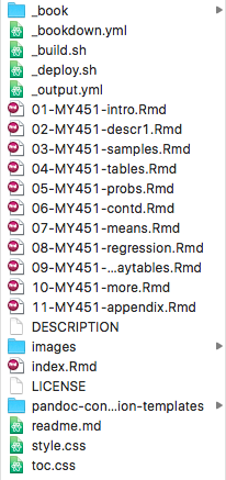
Now you have an exact and complete copy of the project folder on your computer. It should look something like this:
The folder includes the content of the course pack as well as settings files. The files and folder relevant for contributors are:
(1) files ending in .Rmd are the manuscript divided by chapters, and
(2) the folder images/ where image files of figures go that you want to include in the course pack.
The manuscript of class MY464 is stored in files with the extension .Rmd. One file per chapter. That means you'll find twelve Rmd files in your newly "cloned" project folder of this course pack. The very first chapter of a book project is always stored in index.Rmd. In this case that is the preface of this course pack, "Course information". The ten subject chapters plus the appendix are stored in numbered Rmd files. The number of these chapter manuscript files determine the order you want those chapters to be in.
To make changes to the course pack manuscript go ahead and open one of the Rmd files with a text editor of your choice. You can use any editor you prefer or that ships with your operating system. I use Atom, a text editor that is open source and supports syntax highlighting and Git integration. Two features that may come in handy for contributors to this course pack. You can download Atom here.
If you use Atom, I recommend you install the package "language-pfm". That will highlight elements of the manuscript text visually according to the authoring convention this process relies on. Another package you may find useful in order to have your writing experience free from distraction is "Zen". Both packages can be installed going to the menu bar of Atom Editor and clicking "Atom" > "Settings" > "+ Install" on the left-hand sidebar > enter the name of the package you want to install in the search field > hit Enter > find it in the search results that appear below and click "Install". Once you have done that, syntax highlighting will be in effect, no more action needed. To activate the distraction-free "zen" mode for writing, in the menu bar, go to "View" > "Toggle Command Palette" and enter "zen" into the search field that appears. In the search results right below click "Zen: Toggle".
You can further modify the appearance of the Atom Text Editor in its settings under "Themes" in the left-hand sidebar.
For the Rmd files and particularly the tables to display correctly, it is important that soft line wrapping is disabled. If a table looks broken up to you, in the menu bar, go to "View" > "Toggle Command Palette" and enter "wrap" into the search field. Click "Editor: Toggle Soft Wrap" in the search results below.
If you are familiar with how these manuscript files looked before, you'll notice a stark difference. As opposed to the old manuscript files, the new ones before you are visually coherent and easily human-readable. That is because they rely on an authoring convention called Markdown. More specifically, Pandoc-flavored Markdown.
Like HTML or Latex, Markdown is a way to mark elements of text as what we want them to be. Unlike HTML or Latex, however, Markdown requires minimal know-how while affording most of the functionalities of HTML or Latex. The only text elements in the manuscript before you that require knowledge of Latex are equations. Keep reading for an overview of writing in Markdown. You can also find the full documentation of Pandoc-flavored Markdown here.
Headings, headers, or titles are made by putting a hash (#) in front of them and having them be preceded by a blank line.
The number of hashes determines the level of the heading:
...ending of previous paragraph.

# This is a top-level header

## This is a level 2 header

### This is a level 3 header
.
.

###### This is a level 6/bottom-level header
or
# Chapter

## Section

### Subsection

#### Subsubsection
By default, headers will automatically be numbered in the output (the website, the printable, the ebook) according to their level and position in the manuscript. Some headers, however, you may not want to be numbered -- for example level 4-6 headers or headers in the preface or appendix. In order to exclude those from being automatically numbered append {-} like so:
# Appendix {-}
Numbered lists can be created this way:
1. First item
2. Second item
3. Third item
Unnumbered lists can be created this way:
* unnumbered item
  + subitem
    - subsubitem
  + subitem
+ item
  + subitem
Any string of text -- words, phrases, headers, paragraphs -- can be emphasized by bracketing it in asterisks like so:
*Italicize* with a single asterisk before and after.

Make text **bold** with two asterisks.

Text will be ***bold and italic*** in the output with three asterisks.A simple table can look like this:
  Region               Frequency   Proportion       %
  ------------------ ----------- ------------ -------
  Africa                      48        0.310    31.0
  Asia                        44        0.284    28.4
  Europe                      34        0.219    21.9
  Latin America               23        0.148    14.8
  Northern America             2        0.013     1.3
  Oceania                      4        0.026     2.6
  Total                      155        1.000   100.0

  : (\#tab:t-region)Frequency distribution of the region variable in the country data.
You'll notice that the horizontal rule and its breaks determine the number and relative size of rows.
The alignment of a row is determined by where you place the content of the first line in relation to the horizontal rule. It does not matter where exactly you place the remaining content as long as it is within the row. In the output, the entire row will be aligned according to the first line:
Left-aligned   Centered   Right-aligned
------------- ---------- --------------
    0.1              1.0 0.0
Becomes:
A multiline table with cells that take up more than one line can look like the one below. In multiline tables it is crucial that
- the table begins and ends with a row of dashes,
- rows are separated by blank lines, and that
- the bottom row of dashes is followed by a blank line
-------------------------------------------------------------
 Centered   Default           Right Left
  Header    Aligned         Aligned Aligned
----------- ------- --------------- -------------------------
   First    row                12.0 Example of a row that
                                    spans multiple lines.

  Second    row                 5.0 Here's another one. Note
                                    the blank line between
                                    rows.
-------------------------------------------------------------

  : Example of a multiline table.
Captions can be added to tables following the example above. For how to add unique identifiers to tables see "Anchors, Labels, Identifiers and referencing them" below.
Any image file you want to insert in the manuscript needs to be stored in the folder images/ that's inside the project folder.
You can insert a figure -- in other words an image -- by following this format:

Make sure to prepend and follow an image with a blank line. Otherwise it won't get numbered and captioned in the pdf output!It is important that in the manuscript you give the file name without a file extension as shown above and that you provide one and the same image in two file formats: .pdf and .png.
For example, in order to insert into the manuscript a figure "bar_attitude" it needs to read in the manuscript like this:

and the images/ folder needs to include both bar_attitude.pdf and bar_attitude.png. This is to meet the distinct challenges of both print and screen output.
Assuming a figure you made is available in .eps format or .pdf, you can produce a pdf or png file using your operating system's standard picture viewer. On Mac OS X, for example, open an image file with the Preview app and click "File" > "Export..."" > then choose output format PNG > select path to the images/ folder inside the project folder > click "Save".
Equations need to be authored in Latex. In-line equations need to be bracketed with a dollar sign. A blank space is necessary before the opening $ and after the closing $.
Separate equations need to be bracketed with double dollar signs. Again, a blank space is necessary before the opening $$ and after the closing $$.
Separate, labeled and automatically numbered equations need to be bracketed with \begin{equation} and \end{equation} respectively.
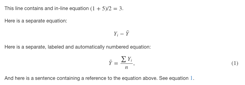
This line contains an in-line equation $(1+5)/2=3$.

Here is a separate equation:

$$Y_{i}-\bar{Y}$$

Here is a separate, labeled and automatically numbered equation:

\begin{equation}
\bar{Y}=\frac{\sum Y_{i}}{n}, \label{eq:example-equation}
\end{equation}

And here is a sentence containing a reference to the equation above. See equation \@ref(eq:example-equation).
In the output it will look like this:
Headers, tables, figures, and equations can be given unique identifiers, also called anchors or labels, that allows you to reference them elsewhere in the manuscript. A unique identifier numbers an item automatically. When you reference that unique identifier elsewhere in the manuscript the dynamically associated number will be shown in the output. At the moment, equations can only be referenced dynamically inside the same manuscript file, in other words, inside the same chapter.
Labelling a header:
# Introduction {unique-identifier}A header can only either be given a unique identifier or be made unnumbered ({-}).
Labelling a table:
To give a unique identifier to a table include it at the very beginning of a table's caption in this format:
: (\#tab:unique-identifier)Caption text with no space between unique identifier and caption text.Labelling a figure:
To give a unique identifier to a figure include it at the very beginning of a figure's caption in this format:
Labelling an equation:
Labelling an equation can be done by including \label{eq:unique-identifier} in the Latex code of the equation. Remember that labelled equations will display in a separate line and automatically numbered and need to be bracketed in \begin{equation} and \end{equation}.
\begin{equation}
\bar{Y}=\frac{\sum Y_{i}}{n} \label{eq:example-equation}
\end{equation}
Any unique identifier can be referenced elsewhere in the manuscript with the expression \@ref(unique-identifier). Make sure to prefix the unique identifier with what you are referencing: tab: for tables, fig: for figures, and eq: for equations; headings take no prefix.
See Section \@ref(c-intro).

See table \@ref(tab:t-region).

See figure \@ref(fig:bar_attitude).

See equation \@ref(eq:example-equation) in this chapter.
Footnotes can be added in-line and will be typeset automatically at the bottom of the page. Follow the following format:
Honeymoon salad is made from lettuce alone and no dressing.^[The Late Show with Stephen Colbert, CBS, September 16, 2016.]If you are familiar with the programming language R you can also use the RStudio application with the "knitr" expansion to author manuscripts. There is no R code used in this MY464 course pack. But you may find R useful for producing complex or dynamic tables or figures in your book project. You can even produce dynamic figures that readers of your book's website can interact with.
You can find documentation for a variation of Markdown that supports R code here.
RStudio can be found and downloaded here.
Documentation for the knitr expansion can be found here.
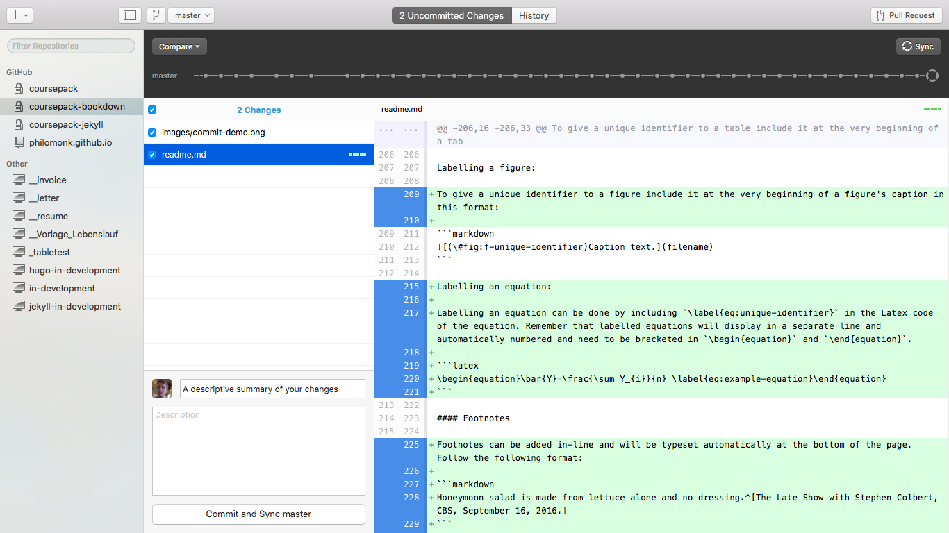
Once you have made and saved changes to any file in the project folder, they will be shown as "uncommitted changes" in your GitHub Desktop app.
In order for you to be able to upload your changes your GitHub account needs to be registered as a contributor to the project's repository. Ask the project repository's administrator for that privilege.
To upload the changed files, which is also called "pushing" changes, go to your GitHub Desktop app. Select this project's repository on the left-hand side where your repositories are listed. Enter a brief description of the changes you made. Click the "Commit" button at the bottom. Depending on your settings GitHub Desktop may upload your changes automatically after clicking "Commit" or you may need to press the "Sync" button at the top right of the app manually.
Your changes will be in effect shortly. This can be within three minutes or thirty minutes depending on the workload of the Travis CI server that does the compiling. Check out https://lse-methodology.github.io/MY464/ and download the pdf printable and epub ebook to view your changes.
-- This prototype was developed by Tobias Pester, September 2016.


