standaRdized is an R package for the calculation of Standardized Index values (SPI, SPEI, SSI,...) on a daily basis. The Standardized Precipitation Index (SPI) was developed by McKee et al (1993) [1] as a monthly indicator for meteorological drought, and has since become one of the most widely used drought indicators. The standardized index procedure has also been applied to time series of the precipitation-evaporation balance (Standardized Precipitation Evapotranspiration Index, SPEI), and streamflow (Standardized Streamflow Index, SSI).
This package provides functions to calculate Standardized Index values on a daily basis in a generalized way: it allows the use of several distributions, aggregation periods, reference periods, and aggregation functions. This allows the calculation of Standardized Index values for a wide range of environmental data (e.g. groundwater levels, temperature,…).
Further details:
standaRdized can be installed from GitHub with:
# install.packages("devtools")
devtools::install_github("WillemMaetens/standaRdized")standaRdized uses xts (eXtensible Time Series) as input and output objects. Some tutorials for working with xts objects can be found here or here.
Load the package with:
library(standaRdized)The package includes example daily rainfall data for the Ukkel station in Belgium (source: ECA&D). This data can be loaded with:
data("Ukkel_RR")The function fprint() can be used to print xts objects or lists of xts objects in a formatted manner. It prints the xtsAttributes where the metadata for time series are stored, and the head and tail of xts time series.
fprint(Ukkel_RR)
#> Attributes:
#> name      :  Ukkel
#> country   :  Belgium
#> element   :  RR
#> unit      :  mm
#> longitude :  4.36638889
#> latitude  :  50.8
#> elevation :  100
#> source    :  ECA&D (ecad.eu)
#>
#> Data:
#>            value
#> 1880-01-01    NA
#> 1880-01-02   0.4
#> 1880-01-03   0.0
#> 1880-01-04   0.0
#> 1880-01-05   0.0
#> ...
#> 2019-02-24     0
#> 2019-02-25     0
#> 2019-02-26     0
#> 2019-02-27     0
#> 2019-02-28    11
Calculating Standardized Indexes on a daily basis requires that monthly total precipitation as in the original definition of the SPI is replaced by the total precipitation over a specific number of days (the aggregation period). Although it is possible to do this for any number of days, the traditional definition of SPI-1 (based on total precipitation for 1 month) and SPI-3 (based on total precipitation for 3 months) is approximated by using a fixed period of 30 days for a month. Hence, SPI-1 represents total precipitation over 30 days, SPI-3 total precipitation over 90 days, etc.
Standardized Index values are calculated by the function standardized.index(). Minimum required arguments for this function are data: an xts object with the input time series (e.g. Ukkel_RR), agg.length: the length of the aggregation period in days and index.out: the output dates for which to calculate the SPI:
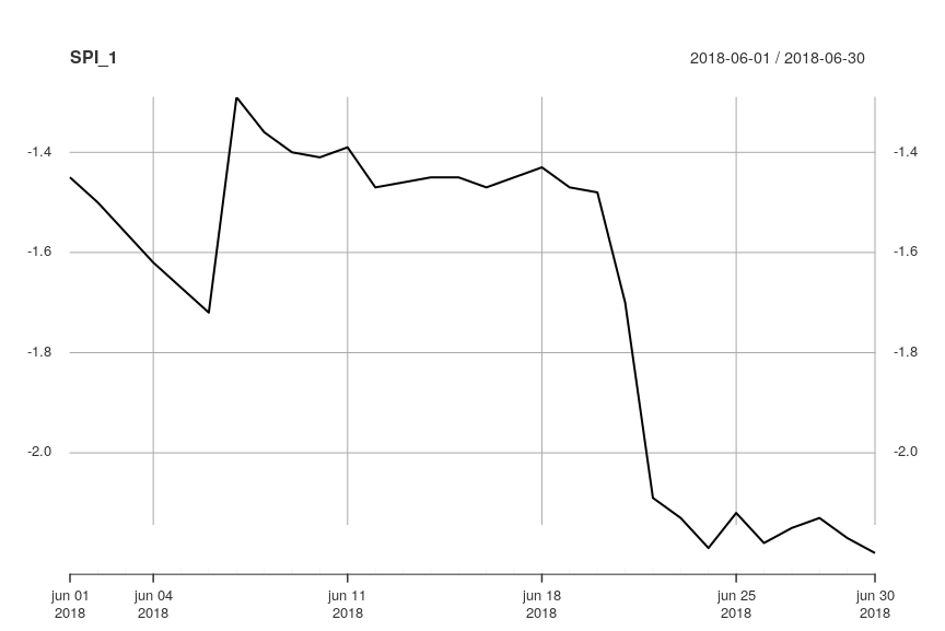
dates <- seq(from = as.Date('2018-06-01'), to = as.Date('2018-06-30'), by = 1)By default, standardized.index uses the gamma distribution and aggregates data using the sum function as these are traditional for the SPI. Hence, the SPI-1 (which has an agg.length of 30 days) for June 2018 is calculated as follows:
SPI_1 <- standardized.index(data = Ukkel_RR, agg.length = 30, index.out = dates)
fprint(SPI_1)
#> Attributes:
#> agg.length        :  30
#> agg.fun           :  sum
#> distr             :  gamma
#> method            :  mle
#> ref.length        :  30
#> ref.na.thres      :  10
#> agg.na.thres      :  10
#> agg.interpolation :  none
#>
#> Data:
#>            value
#> 2018-06-01 -1.45
#> 2018-06-02 -1.50
#> 2018-06-03 -1.56
#> 2018-06-04 -1.62
#> 2018-06-05 -1.67
#> ...
#> 2018-06-26 -2.18
#> 2018-06-27 -2.15
#> 2018-06-28 -2.13
#> 2018-06-29 -2.17
#> 2018-06-30 -2.20
plot(SPI_1)
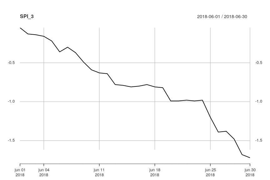
To calculate the SPI-3 (which has an agg.length of 90 days), just modify the agg.length argument:
SPI_3 <- standardized.index(data = Ukkel_RR, agg.length = 90, index.out = dates)
fprint(SPI_3)
#> Attributes:
#> agg.length        :  90
#> agg.fun           :  sum
#> distr             :  gamma
#> method            :  mle
#> ref.length        :  30
#> ref.na.thres      :  10
#> agg.na.thres      :  10
#> agg.interpolation :  none
#>
#> Data:
#>            value
#> 2018-06-01 -0.05
#> 2018-06-02 -0.13
#> 2018-06-03 -0.14
#> 2018-06-04 -0.16
#> 2018-06-05 -0.22
#> ...
#> 2018-06-26 -1.39
#> 2018-06-27 -1.38
#> 2018-06-28 -1.48
#> 2018-06-29 -1.68
#> 2018-06-30 -1.72
plot(SPI_3)
By default, standardized.index uses the entire data object as reference data to determine the reference data on which a distribution is fitted. However, it is possible to provide a seperate ref.data xts that will be used to determine the reference data. This allows the calculation of Standardized Index values for time series of limited length by using another, longer, time series from a nearby station as reference data. This is how the SPI values published by the Flanders Evironment Agency at waterinfo.be are calculated: the SPI-1 and SPI-3 for 43 raingauges with data from 2004 onwards are calculated by using the long term daily rainfall record at RMI's Ukkel station as reference data.
Furthermore, the ref.years and ref.length arguments allow to set which period of data to use as reference period. By default (ref.years = NULL), the full dataset length of ref.data is used, but you can provide specific years to be used as reference period. For instance, the European Drought Observatory uses the years 1981-2010 as reference period:
SPI_1 <- standardized.index(data = Ukkel_RR, agg.length = 30, index.out = dates, ref.years = seq(1981, 2010))
fprint(SPI_1)
#> Attributes:
#> agg.length        :  30
#> agg.fun           :  sum
#> distr             :  gamma
#> method            :  mle
#> ref.years         :  1981, 1982, 1983, 1984, 1985, 1986, 1987, 1988,... [truncated]
#> ref.length        :  30
#> ref.na.thres      :  10
#> agg.na.thres      :  10
#> agg.interpolation :  none
#>
#> Data:
#>            value
#> 2018-06-01 -2.10
#> 2018-06-02 -2.15
#> 2018-06-03 -2.45
#> 2018-06-04 -2.58
#> 2018-06-05 -2.53
#> ...
#> 2018-06-26 -2.22
#> 2018-06-27 -2.15
#> 2018-06-28 -2.11
#> 2018-06-29 -2.16
#> 2018-06-30 -2.20
Alternatively, instead of a set reference period, a set number of years preceding the date for which the Standardized Index is calculated can be used by setting ref.years = NA and specifying ref.length as a set number of years (by default, this is 30). This is the setting used by VMM to calculate the SPI values shown on waterinfo.be.
SPI_1 <- standardized.index(data = Ukkel_RR, agg.length = 30, index.out = dates, ref.years = NA, ref.length = 30)
fprint(SPI_1)
#> Attributes:
#> agg.length        :  30
#> agg.fun           :  sum
#> distr             :  gamma
#> method            :  mle
#> ref.years         :  NA
#> ref.length        :  30
#> ref.na.thres      :  10
#> agg.na.thres      :  10
#> agg.interpolation :  none
#>
#> Data:
#>            value
#> 2018-06-01 -1.89
#> 2018-06-02 -1.84
#> 2018-06-03 -2.06
#> 2018-06-04 -2.16
#> 2018-06-05 -2.21
#> ...
#> 2018-06-26    NA
#> 2018-06-27    NA
#> 2018-06-28    NA
#> 2018-06-29    NA
#> 2018-06-30    NA
Note how this introduces NA values in the output as the data for more recent years in the Ukkel_RR series has not yet been consolidated and the function's default tolerance for 10% missing data in the aggregation period or reference period is exceeded.
For more information on the calculation procedure for Standardized Index values, see: Standardized Index calculation.
For more information on the package's functions, see: function help.
[1] McKee, T.B., Doesken, N.J. and Kleist, J., 1993. The relationship of drought frequency and duration to time scales. In Proceedings of the 8th Conference on Applied Climatology, American Meteorological Society. Vol. 17, No. 22, pp. 179-183.

