UrbanInstitute / syntheval

syntheval

syntheval makes it simple to evaluate the utility and disclosure risks of synthetic data. The package is designed to work with postsynth objects from library(tidysynthesis) but also works well with any data frame in R.

Note: library(tidysynthesis) is currently under private development but will be made public in the future.

Navigation

• Installation
• Utility Metrics
  • Proportions
  • Means and totals
  • Percentiles
  • KS Distance
  • Co-Occurrence
  • Correlations
  • Coefficient overlap
  • Discriminant-based metrics
• Additional Functionality
  • Grouping
  • Weighting

Installation

install.packages("remotes")
remotes::install_github("UrbanInstitute/syntheval")

Utility Metrics

library(tidyverse)
library(syntheval)

Setup

The following examples demonstrate utility and disclosure risk metrics using synthetic data based on the Palmer Penguins dataset. library(syntheval) contains three built-in data sets:

• penguins_conf: Pre-processed penguins data that were passed into the synthesizer.
• penguins_postsynth: A postsynth object synthesized from penguins using library(tidysynthesis).
• penguins_syn_df: A data frame pulled from penguins_postsynth. This is used to demonstrate how library(syntheval) works with output from a synthesizer different than library(tidysynthesis).

Functions like util_proportions() and util_moments() have different behaviors for postsynth objects and data frames. By default, they only show synthesized variables for postsynth objects and show all common variables for data frames. The common_vars and synth_vars arguments can change this behavior.

Proportions

util_proportions() compares the proportions of classes from categorical variables in the original data and synthetic data.

util_proportions(
  postsynth = penguins_postsynth, 
  data = penguins_conf
)

# A tibble: 2 × 5
# Groups:   variable [1]
  variable class  synthetic original difference
  <chr>    <fct>      <dbl>    <dbl>      <dbl>
1 sex      female     0.529    0.495     0.0330
2 sex      male       0.471    0.505    -0.0330

All common variables are shown when using a data frame.

util_proportions(
  postsynth = penguins_syn_df, 
  data = penguins_conf
)

# A tibble: 8 × 5
# Groups:   variable [3]
  variable class     synthetic original difference
  <chr>    <fct>         <dbl>    <dbl>      <dbl>
1 island   Biscoe        0.465    0.489    -0.0240
2 island   Dream         0.414    0.369     0.0450
3 island   Torgersen     0.120    0.141    -0.0210
4 sex      female        0.529    0.495     0.0330
5 sex      male          0.471    0.505    -0.0330
6 species  Adelie        0.459    0.438     0.0210
7 species  Chinstrap     0.234    0.204     0.0300
8 species  Gentoo        0.306    0.357    -0.0511

Means and Totals

util_moments() compares the counts, means, standard deviations, skewnesses, and kurtoses of the original data and synthetic data.

util_moments(
  postsynth = penguins_postsynth, 
  data = penguins_conf
)

# A tibble: 20 × 6
   variable        statistic original synthetic difference proportion_difference
   <fct>           <fct>        <dbl>     <dbl>      <dbl>                 <dbl>
 1 bill_length_mm  count      3.33e+2  333          0                    0      
 2 bill_length_mm  mean       4.40e+1   43.5       -0.502               -0.0114 
 3 bill_length_mm  sd         5.47e+0    5.54       0.0723               0.0132 
 4 bill_length_mm  skewness   4.51e-2    0.0646     0.0195               0.432  
 5 bill_length_mm  kurtosis  -8.88e-1   -0.948     -0.0598               0.0674 
 6 bill_depth_mm   count      3.33e+2  333          0                    0      
 7 bill_depth_mm   mean       1.72e+1   17.3        0.122                0.00712
 8 bill_depth_mm   sd         1.97e+0    1.89      -0.0762              -0.0387 
 9 bill_depth_mm   skewness  -1.49e-1   -0.278     -0.129                0.867  
10 bill_depth_mm   kurtosis  -8.97e-1   -0.742      0.155               -0.172  
11 flipper_length… count      3.33e+2  333          0                    0      
12 flipper_length… mean       2.01e+2  199.        -1.70                -0.00847
13 flipper_length… sd         1.40e+1   13.9       -0.135               -0.00961
14 flipper_length… skewness   3.59e-1    0.611      0.253                0.705  
15 flipper_length… kurtosis  -9.65e-1   -0.704      0.261               -0.270  
16 body_mass_g     count      3.33e+2  333          0                    0      
17 body_mass_g     mean       4.21e+3 4162.       -45.0                 -0.0107 
18 body_mass_g     sd         8.05e+2  783.       -22.3                 -0.0277 
19 body_mass_g     skewness   4.70e-1    0.655      0.185                0.394  
20 body_mass_g     kurtosis  -7.40e-1   -0.388      0.353               -0.477  

util_totals() is similar to util_moments() but looks at counts and totals.

util_totals(
  postsynth = penguins_postsynth, 
  data = penguins_conf
)

# A tibble: 8 × 6
  variable         statistic original synthetic difference proportion_difference
  <fct>            <fct>        <dbl>     <dbl>      <dbl>                 <dbl>
1 bill_length_mm   count         333       333         0                 0      
2 bill_length_mm   total       14650.    14483.     -167.               -0.0114 
3 bill_depth_mm    count         333       333         0                 0      
4 bill_depth_mm    total        5716.     5757.       40.7               0.00712
5 flipper_length_… count         333       333         0                 0      
6 flipper_length_… total       66922     66355      -567                -0.00847
7 body_mass_g      count         333       333         0                 0      
8 body_mass_g      total     1400950   1385950    -15000                -0.0107 

Percentiles

util_percentiles() compares percentiles from the original data and synthetic data. The default percentiles are c(0.1, 0.5, 0.9) and can be easily overwritten.

util_percentiles(
  postsynth = penguins_postsynth, 
  data = penguins_conf,
  probs = c(0.5, 0.8)
)

# A tibble: 8 × 6
      p variable          original synthetic difference proportion_difference
  <dbl> <fct>                <dbl>     <dbl>      <dbl>                 <dbl>
1   0.5 bill_length_mm        44.5      43.5    -1                   -0.0225 
2   0.8 bill_length_mm        49.5      49.1    -0.440               -0.00889
3   0.5 bill_depth_mm         17.3      17.5     0.200                0.0116 
4   0.8 bill_depth_mm         18.9      19.0     0.0600               0.00317
5   0.5 flipper_length_mm    197       195      -2                   -0.0102 
6   0.8 flipper_length_mm    215       214      -1                   -0.00465
7   0.5 body_mass_g         4050      3950    -100                   -0.0247 
8   0.8 body_mass_g         4990      4850    -140                   -0.0281 

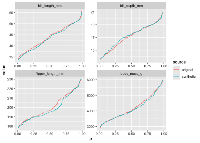
The functions are designed to work well with library(ggplot2).

util_percentiles(
  postsynth = penguins_postsynth, 
  data = penguins_conf,
  probs = seq(0.01, 0.99, 0.01)
) |>
  pivot_longer(
    cols = c(original, synthetic),
    names_to = "source",
    values_to = "value"
  ) |>
  ggplot(aes(x = p, y = value, color = source)) +
  geom_line() +
  facet_wrap(~ variable, scales = "free")

KS Distance

util_ks_distance() shows the Kolmogorov-Smirnov distance between the original distribution and synthetic distribution for numeric variables. The function also returns the point(s) of the maximum distance.

util_ks_distance(
  postsynth = penguins_syn_df, 
  data = penguins_conf
)

# A tibble: 14 × 3
   variable           value      D
   <chr>              <dbl>  <dbl>
 1 bill_length_mm      38.7 0.0601
 2 bill_depth_mm       16.7 0.0511
 3 bill_depth_mm       16.7 0.0511
 4 bill_depth_mm       16.8 0.0511
 5 bill_depth_mm       16.8 0.0511
 6 flipper_length_mm  196.  0.0781
 7 flipper_length_mm  196.  0.0781
 8 flipper_length_mm  197.  0.0781
 9 flipper_length_mm  197.  0.0781
10 flipper_length_mm  197.  0.0781
11 body_mass_g       4359.  0.0480
12 body_mass_g       4370.  0.0480
13 body_mass_g       4381.  0.0480
14 body_mass_g       4392.  0.0480

Co-Occurrence

util_co_occurrence() differences the lower triangles of co-occurrence matrices calculated on numeric variables in the original data and synthetic data.

co_occurrence <- util_co_occurrence(
  postsynth = penguins_postsynth, 
  data = penguins_conf
)

co_occurrence$co_occurrence_difference

                  bill_length_mm bill_depth_mm flipper_length_mm body_mass_g
bill_length_mm                NA            NA                NA          NA
bill_depth_mm                  0            NA                NA          NA
flipper_length_mm              0             0                NA          NA
body_mass_g                    0             0                 0          NA

The function returns the MAE for co-occurrences, which provides a sense of the median error between the original and synthetic data. The function also returns the RMSE for co-occurrences, which provides a sense of the average error between the original data and synthetic data.

co_occurrence$co_occurrence_difference_mae

[1] 0

co_occurrence$co_occurrence_difference_rmse

[1] 0

All observations have non-zero bill_length_mm, bill_depth_mm, flipper_length_mm, and body_mass_g. util_co_occurrence() is most useful for economic variables like income and wealth where 0 is a common value.

Correlations

util_corr_fit() differences the lower triangles of correlation matrices calculated on numeric variables in the original data and synthetic data.

corr_fit <- util_corr_fit(
  postsynth = penguins_postsynth, 
  data = penguins_conf
)

round(corr_fit$correlation_difference, digits = 3)

                  bill_length_mm bill_depth_mm flipper_length_mm body_mass_g
bill_length_mm                NA            NA                NA          NA
bill_depth_mm             -0.069            NA                NA          NA
flipper_length_mm         -0.003        -0.048                NA          NA
body_mass_g                0.031        -0.011             -0.08          NA

The function returns the MAE for correlation coefficients, which provides a sense of the median error between the original and synthetic data. The function also returns the RMSE for the correlation coefficients, which provides a sense of the average error between the original synthetic data.

corr_fit$correlation_difference_mae

[1] 0.04034565

corr_fit$correlation_difference_rmse

[1] 0.04922324

Coefficient Overlap

util_ci_overlap() compares a linear regression models estimated on the original data and synthetic data. formula specifies the functional form of the regression model.

ci_overlap <- util_ci_overlap(
  postsynth = penguins_postsynth, 
  data = penguins_conf,
  formula = body_mass_g ~ bill_length_mm  + sex
)

$ci_overlap() summarizes each coefficient including how much the confidence intervals overlap, if the signs match, and if the statistical significance matches.

ci_overlap$ci_overlap 

# A tibble: 3 × 8
  term    overlap coef_diff std_coef_diff sign_match significance_match ss_match
  <chr>     <dbl>     <dbl>         <dbl> <lgl>      <lgl>              <lgl>   
1 (Inter…   0.963   -27.8         -0.0978 TRUE       TRUE               TRUE    
2 bill_l…   0.965     0.917        0.138  TRUE       TRUE               TRUE    
3 sexmale   0.951   -14.0         -0.192  TRUE       TRUE               TRUE    
# ℹ 1 more variable: sso_match <lgl>

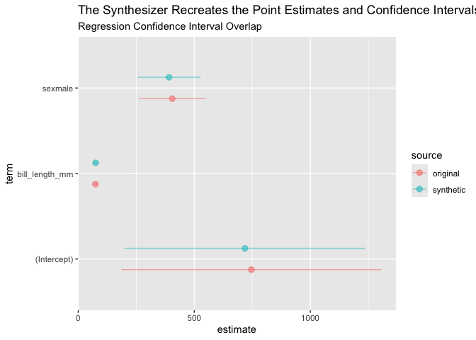
$coefficient provides detail for each coefficient and is useful for data visualization.

ci_overlap$coefficient

# A tibble: 6 × 8
  source    term        estimate std.error statistic  p.value conf.low conf.high
  <chr>     <chr>          <dbl>     <dbl>     <dbl>    <dbl>    <dbl>     <dbl>
1 original  (Intercept)    746.     285.        2.62 9.22e- 3    186.     1306. 
2 original  bill_lengt…     74.0      6.67     11.1  1.51e-24     60.9      87.1
3 original  sexmale        405.      72.8       5.57 5.43e- 8    262.      548. 
4 synthetic (Intercept)    718.     264.        2.72 6.77e- 3    200.     1237. 
5 synthetic bill_lengt…     74.9      6.25     12.0  8.98e-28     62.7      87.2
6 synthetic sexmale        391.      69.2       5.65 3.42e- 8    255.      527. 

ci_overlap$coefficient |>
  ggplot(aes(x = estimate, xmin = conf.low, xmax = conf.high, y = term, color = source)) +
  geom_pointrange(alpha = 0.5, position = position_dodge(width = 0.5)) +
  labs(
    title = "The Synthesizer Recreates the Point Estimates and Confidence Intervals",
    subtitle = "Regression Confidence Interval Overlap"
  )

Discriminant-Based Metrics

Discriminant-based metrics build models to predict if an observation is original or synthetic and then evaluate those model predictions. Ideally, it should be difficult for a model to distinguish, or discriminate, between original observations and synthetic observations.

• Any classification model that generates probabilities from library(tidymodels) can be used to generate propensities (the estimated probability than observation is synthetic).
• By default, the code creates a training/testing split and returns separate metrics for each split. This can be turned off with split = FALSE.
• The code can handle hyperparameter tuning.
• After calculating propensities, the code can calculate ROC AUC, SPECKS, pMSE, and pMSE ratio.

Example Using Decision Trees

Discriminant-based metrics are built a discrimination object created by discrimination().

disc1 <- discrimination(postsynth = penguins_postsynth, data = penguins_conf)

Next, we use library(tidymodels) to specify a model. We recommend the tidymodels tutorial to learn more.

library(tidymodels)

rpart_rec <- recipe(
  .source_label ~ ., 
  data = disc1$combined_data
)

rpart_mod <- decision_tree(cost_complexity = 0.01) |>
  set_mode(mode = "classification") |>
  set_engine(engine = "rpart")

Next, we fit the model to the data to generate predicted probabilities.

disc1 <- disc1 |>
  add_propensities(
    recipe = rpart_rec,
    spec = rpart_mod
  ) 

At this point, we can use

• add_discriminator_auc() to add the ROC AUC for the predicted probabilities
• add_specks() to add SPECKS for the predicted probabilities
• add_pmse() to add pMSE for the predicted probabilities
• add_pmse_ratio(times = 25) to add the pMSE ratio using the pMSE model and 25 bootstrap samples

disc1 |>
  add_discriminator_auc() |>
  add_specks() |>
  add_pmse() |>
  add_pmse_ratio(times = 25)

$combined_data
# A tibble: 666 × 8
   .source_label species island    sex    bill_length_mm bill_depth_mm
   <fct>         <fct>   <fct>     <fct>           <dbl>         <dbl>
 1 original      Adelie  Torgersen male             39.1          18.7
 2 original      Adelie  Torgersen female           39.5          17.4
 3 original      Adelie  Torgersen female           40.3          18  
 4 original      Adelie  Torgersen female           36.7          19.3
 5 original      Adelie  Torgersen male             39.3          20.6
 6 original      Adelie  Torgersen female           38.9          17.8
 7 original      Adelie  Torgersen male             39.2          19.6
 8 original      Adelie  Torgersen female           41.1          17.6
 9 original      Adelie  Torgersen male             38.6          21.2
10 original      Adelie  Torgersen male             34.6          21.1
# ℹ 656 more rows
# ℹ 2 more variables: flipper_length_mm <dbl>, body_mass_g <dbl>

$propensities
# A tibble: 666 × 10
   .pred_synthetic .source_label .sample  species island    sex   bill_length_mm
             <dbl> <fct>         <chr>    <fct>   <fct>     <fct>          <dbl>
 1           0.290 original      training Adelie  Torgersen male            39.1
 2           0.290 original      training Adelie  Torgersen fema…           39.5
 3           0.290 original      training Adelie  Torgersen fema…           40.3
 4           0.656 original      training Adelie  Torgersen fema…           36.7
 5           0.290 original      testing  Adelie  Torgersen male            39.3
 6           0.290 original      training Adelie  Torgersen fema…           38.9
 7           0.290 original      testing  Adelie  Torgersen male            39.2
 8           0.290 original      training Adelie  Torgersen fema…           41.1
 9           0.290 original      testing  Adelie  Torgersen male            38.6
10           0.656 original      training Adelie  Torgersen male            34.6
# ℹ 656 more rows
# ℹ 3 more variables: bill_depth_mm <dbl>, flipper_length_mm <dbl>,
#   body_mass_g <dbl>

$discriminator
══ Workflow [trained] ══════════════════════════════════════════════════════════
Preprocessor: Recipe
Model: decision_tree()

── Preprocessor ────────────────────────────────────────────────────────────────
0 Recipe Steps

── Model ───────────────────────────────────────────────────────────────────────
n= 498 

node), split, n, loss, yval, (yprob)
      * denotes terminal node

   1) root 498 249 synthetic (0.5000000 0.5000000)  
     2) bill_length_mm< 38.25 115  46 synthetic (0.6000000 0.4000000)  
       4) body_mass_g>=3187.5 90  31 synthetic (0.6555556 0.3444444) *
       5) body_mass_g< 3187.5 25  10 original (0.4000000 0.6000000)  
        10) bill_depth_mm>=17.6 11   4 synthetic (0.6363636 0.3636364) *
        11) bill_depth_mm< 17.6 14   3 original (0.2142857 0.7857143) *
     3) bill_length_mm>=38.25 383 180 original (0.4699739 0.5300261)  
       6) island=Biscoe,Dream 352 171 original (0.4857955 0.5142045)  
        12) body_mass_g< 3375 28   9 synthetic (0.6785714 0.3214286) *
        13) body_mass_g>=3375 324 152 original (0.4691358 0.5308642)  
          26) bill_length_mm>=41.2 280 136 original (0.4857143 0.5142857)  
            52) flipper_length_mm< 189.5 18   4 synthetic (0.7777778 0.2222222) *
            53) flipper_length_mm>=189.5 262 122 original (0.4656489 0.5343511)  
             106) body_mass_g>=3587.5 252 120 original (0.4761905 0.5238095)  
               212) flipper_length_mm< 192.5 15   5 synthetic (0.6666667 0.3333333) *
               213) flipper_length_mm>=192.5 237 110 original (0.4641350 0.5358650)  
                 426) body_mass_g>=4287.5 185  91 original (0.4918919 0.5081081)  
                   852) bill_length_mm>=50.45 40  15 synthetic (0.6250000 0.3750000)  
                    1704) bill_length_mm< 52.35 30   8 synthetic (0.7333333 0.2666667) *
                    1705) bill_length_mm>=52.35 10   3 original (0.3000000 0.7000000) *
                   853) bill_length_mm< 50.45 145  66 original (0.4551724 0.5448276)  
                    1706) bill_length_mm< 47.05 80  37 synthetic (0.5375000 0.4625000)  
                      3412) bill_length_mm>=46.65 8   1 synthetic (0.8750000 0.1250000) *
                      3413) bill_length_mm< 46.65 72  36 synthetic (0.5000000 0.5000000)  
                        6826) body_mass_g< 5025 58  26 synthetic (0.5517241 0.4482759) *
                        6827) body_mass_g>=5025 14   4 original (0.2857143 0.7142857) *
                    1707) bill_length_mm>=47.05 65  23 original (0.3538462 0.6461538)  
                      3414) bill_depth_mm>=15.65 28  14 synthetic (0.5000000 0.5000000)  
                        6828) body_mass_g< 5525 12   3 synthetic (0.7500000 0.2500000) *
                        6829) body_mass_g>=5525 16   5 original (0.3125000 0.6875000) *
                      3415) bill_depth_mm< 15.65 37   9 original (0.2432432 0.7567568) *
                 427) body_mass_g< 4287.5 52  19 original (0.3653846 0.6346154)  
                   854) bill_depth_mm>=19.65 12   4 synthetic (0.6666667 0.3333333) *
                   855) bill_depth_mm< 19.65 40  11 original (0.2750000 0.7250000) *
             107) body_mass_g< 3587.5 10   2 original (0.2000000 0.8000000) *
          27) bill_length_mm< 41.2 44  16 original (0.3636364 0.6363636)  
            54) bill_depth_mm>=18.95 17   7 synthetic (0.5882353 0.4117647) *
            55) bill_depth_mm< 18.95 27   6 original (0.2222222 0.7777778) *
       7) island=Torgersen 31   9 original (0.2903226 0.7096774) *

$discriminator_auc
# A tibble: 2 × 4
  .sample  .metric .estimator .estimate
  <fct>    <chr>   <chr>          <dbl>
1 training roc_auc binary         0.726
2 testing  roc_auc binary         0.449

$pmse
# A tibble: 2 × 4
  .source   .pmse .null_pmse .pmse_ratio
  <fct>     <dbl>      <dbl>       <dbl>
1 training 0.0417     0.0374        1.12
2 testing  0.0450     0.0361        1.25

$specks
# A tibble: 2 × 2
  .source  .specks
  <fct>      <dbl>
1 training   0.382
2 testing    0.107

attr(,"class")
[1] "discrimination"

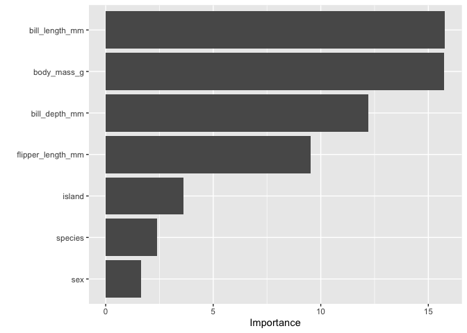
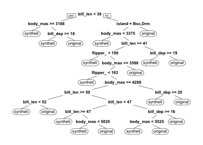
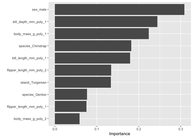
Finally, we can look at variable importance and the decision tree from our discriminator.

library(vip)
library(rpart.plot)

disc1$discriminator |> 
  extract_fit_parsnip() |> 
  vip()

disc1$discriminator$fit$fit$fit |>
  prp()

Warning: Cannot retrieve the data used to build the model (so cannot determine roundint and is.binary for the variables).
To silence this warning:
    Call prp with roundint=FALSE,
    or rebuild the rpart model with model=TRUE.

Example Using Regularized Regression

Let’s repeat the workflow from above with LASSO logistic regression and hyperparameter tuning.

# create discrimination
disc2 <- discrimination(postsynth = penguins_postsynth, data = penguins_conf)

# create a recipe that includes 2nd-degree polynomials, dummy variables, and
# standardization
lasso_rec <- recipe(
  .source_label ~ ., 
  data = disc2$combined_data
) |>
  step_poly(all_numeric_predictors(), degree = 2) |>
  step_dummy(all_nominal_predictors()) |>
  step_normalize(all_predictors())

# create the model
lasso_mod <- logistic_reg(
  penalty = tune(), 
  mixture = 1
) |>
  set_engine(engine = "glmnet") |>
  set_mode(mode = "classification")

# create a tuning grid
lasso_grid <- grid_regular(penalty(), levels = 10)

# add the propensities
disc2 <- disc2 |>
  add_propensities_tuned(
    recipe = lasso_rec,
    spec = lasso_mod,
    grid = lasso_grid
  ) 

# calculate metrics
disc2 |>
  add_discriminator_auc() |>
  add_specks() |>
  add_pmse() |>
  add_pmse_ratio(times = 25)

$combined_data
# A tibble: 666 × 8
   .source_label species island    sex    bill_length_mm bill_depth_mm
   <fct>         <fct>   <fct>     <fct>           <dbl>         <dbl>
 1 original      Adelie  Torgersen male             39.1          18.7
 2 original      Adelie  Torgersen female           39.5          17.4
 3 original      Adelie  Torgersen female           40.3          18  
 4 original      Adelie  Torgersen female           36.7          19.3
 5 original      Adelie  Torgersen male             39.3          20.6
 6 original      Adelie  Torgersen female           38.9          17.8
 7 original      Adelie  Torgersen male             39.2          19.6
 8 original      Adelie  Torgersen female           41.1          17.6
 9 original      Adelie  Torgersen male             38.6          21.2
10 original      Adelie  Torgersen male             34.6          21.1
# ℹ 656 more rows
# ℹ 2 more variables: flipper_length_mm <dbl>, body_mass_g <dbl>

$propensities
# A tibble: 666 × 10
   .pred_synthetic .source_label .sample  species island    sex   bill_length_mm
             <dbl> <fct>         <chr>    <fct>   <fct>     <fct>          <dbl>
 1           0.439 original      testing  Adelie  Torgersen male            39.1
 2           0.483 original      testing  Adelie  Torgersen fema…           39.5
 3           0.461 original      training Adelie  Torgersen fema…           40.3
 4           0.499 original      training Adelie  Torgersen fema…           36.7
 5           0.443 original      training Adelie  Torgersen male            39.3
 6           0.511 original      training Adelie  Torgersen fema…           38.9
 7           0.416 original      testing  Adelie  Torgersen male            39.2
 8           0.492 original      training Adelie  Torgersen fema…           41.1
 9           0.456 original      training Adelie  Torgersen male            38.6
10           0.447 original      training Adelie  Torgersen male            34.6
# ℹ 656 more rows
# ℹ 3 more variables: bill_depth_mm <dbl>, flipper_length_mm <dbl>,
#   body_mass_g <dbl>

$discriminator
══ Workflow [trained] ══════════════════════════════════════════════════════════
Preprocessor: Recipe
Model: logistic_reg()

── Preprocessor ────────────────────────────────────────────────────────────────
3 Recipe Steps

• step_poly()
• step_dummy()
• step_normalize()

── Model ───────────────────────────────────────────────────────────────────────

Call:  glmnet::glmnet(x = maybe_matrix(x), y = y, family = "binomial",      alpha = ~1) 

   Df %Dev   Lambda
1   0 0.00 0.047070
2   1 0.11 0.042890
3   1 0.20 0.039080
4   1 0.27 0.035600
5   2 0.37 0.032440
6   2 0.48 0.029560
7   3 0.57 0.026930
8   3 0.65 0.024540
9   4 0.74 0.022360
10  5 0.85 0.020370
11  6 0.97 0.018560
12  6 1.09 0.016920
13  6 1.20 0.015410
14  6 1.29 0.014040
15  6 1.36 0.012800
16  6 1.42 0.011660
17  6 1.48 0.010620
18  6 1.52 0.009679
19  7 1.56 0.008820
20  8 1.60 0.008036
21  8 1.64 0.007322
22  8 1.67 0.006672
23  8 1.69 0.006079
24  9 1.73 0.005539
25  9 1.79 0.005047
26  9 1.84 0.004599
27 10 1.88 0.004190
28 10 1.91 0.003818
29 11 1.94 0.003479
30 11 1.96 0.003170
31 11 1.98 0.002888
32 11 2.00 0.002631
33 11 2.01 0.002398
34 12 2.03 0.002185
35 12 2.04 0.001991
36 12 2.05 0.001814
37 12 2.06 0.001653
38 12 2.06 0.001506
39 13 2.07 0.001372
40 13 2.08 0.001250
41 13 2.08 0.001139
42 13 2.09 0.001038
43 13 2.09 0.000946
44 13 2.09 0.000862
45 13 2.10 0.000785
46 13 2.10 0.000715

...
and 5 more lines.

$discriminator_auc
# A tibble: 2 × 4
  .sample  .metric .estimator .estimate
  <fct>    <chr>   <chr>          <dbl>
1 training roc_auc binary         0.589
2 testing  roc_auc binary         0.428

$pmse
# A tibble: 2 × 4
  .source    .pmse .null_pmse .pmse_ratio
  <fct>      <dbl>      <dbl>       <dbl>
1 training 0.00385    0.00272        1.41
2 testing  0.00413    0.00280        1.47

$specks
# A tibble: 2 × 2
  .source  .specks
  <fct>      <dbl>
1 training   0.137
2 testing    0.131

attr(,"class")
[1] "discrimination"

# look at variable importance
library(vip)

disc2$discriminator |> 
  extract_fit_parsnip() |> 
  vip()

Additional Functionality

Grouping

Many utility metrics include a group_by argument to group the metrics by group during calculation. For example, this code calculates moments by species.

util_moments(
  postsynth = penguins_postsynth, 
  data = penguins_conf,
  group_by = species
)

# A tibble: 60 × 7
   species   variable       statistic original synthetic difference
   <fct>     <fct>          <fct>        <dbl>     <dbl>      <dbl>
 1 Adelie    bill_length_mm count      146       153          7    
 2 Chinstrap bill_length_mm count       68        78         10    
 3 Gentoo    bill_length_mm count      119       102        -17    
 4 Adelie    bill_length_mm mean        38.8      38.5       -0.294
 5 Chinstrap bill_length_mm mean        48.8      47.3       -1.56 
 6 Gentoo    bill_length_mm mean        47.6      48.0        0.475
 7 Adelie    bill_length_mm sd           2.66      2.93       0.267
 8 Chinstrap bill_length_mm sd           3.34      3.07      -0.273
 9 Gentoo    bill_length_mm sd           3.11      3.40       0.299
10 Adelie    bill_length_mm skewness     0.156     0.505      0.349
# ℹ 50 more rows
# ℹ 1 more variable: proportion_difference <dbl>

Weighting

Many utility metrics include a weight_var argument to use weighted statistics during calculation. For example, this code weights the moments by the body weight of the penguins.

util_moments(
  postsynth = penguins_postsynth, 
  data = penguins_conf,
  weight_var = body_mass_g
)

# A tibble: 20 × 6
   variable        statistic original synthetic difference proportion_difference
   <fct>           <fct>        <dbl>     <dbl>      <dbl>                 <dbl>
 1 bill_length_mm  count      1.40e+6   1.39e+6   -1.5 e+4              -0.0107 
 2 bill_length_mm  mean       4.46e+1   4.41e+1   -4.71e-1              -0.0106 
 3 bill_length_mm  sd         5.38e+0   5.54e+0    1.60e-1               0.0297 
 4 bill_length_mm  skewness  -7.39e-2  -5.74e-2    1.64e-2              -0.222  
 5 bill_length_mm  kurtosis  -7.89e-1  -9.15e-1   -1.26e-1               0.160  
 6 bill_depth_mm   count      1.40e+6   1.39e+6   -1.5 e+4              -0.0107 
 7 bill_depth_mm   mean       1.70e+1   1.71e+1    1.28e-1               0.00754
 8 bill_depth_mm   sd         2.01e+0   1.94e+0   -7.07e-2              -0.0351 
 9 bill_depth_mm   skewness   1.05e-2  -1.37e-1   -1.47e-1             -14.0    
10 bill_depth_mm   kurtosis  -1.00e+0  -9.17e-1    8.70e-2              -0.0867 
11 flipper_length… count      1.40e+6   1.39e+6   -1.5 e+4              -0.0107 
12 flipper_length… mean       2.03e+2   2.01e+2   -1.97e+0              -0.00970
13 flipper_length… sd         1.44e+1   1.46e+1    1.60e-1               0.0111 
14 flipper_length… skewness   1.48e-1   3.99e-1    2.51e-1               1.70   
15 flipper_length… kurtosis  -1.14e+0  -1.04e+0    1.08e-1              -0.0940 
16 body_mass_g     count      1.40e+6   1.39e+6   -1.5 e+4              -0.0107 
17 body_mass_g     mean       4.36e+3   4.31e+3   -5.19e+1              -0.0119 
18 body_mass_g     sd         8.26e+2   8.17e+2   -9.84e+0              -0.0119 
19 body_mass_g     skewness   2.69e-1   4.64e-1    1.95e-1               0.724  
20 body_mass_g     kurtosis  -9.70e-1  -7.26e-1    2.44e-1              -0.251  

Most commonly, weight_var is used when synthesizing data from surveys.

Getting Help

Contact Aaron R. Williams with feedback or questions.