German Traffic Sign Classification Deep Neural Networks
Build a Traffic Sign Recognition Project
The goals / steps of this project are the following:
- Load the data set (see below for links to the project data set)
- Explore, summarize and visualize the data set
- Design, train and test a model architecture
- Use the model to make predictions on new images
- Analyze the softmax probabilities of the new images
Introduction
1. This project utilizes Deep Neural Networks and Convolutional Neural Networks which is derived from traditional LeNet and Multiscale Convolutional Neural Network. The dataset can be retrived from German Traffic Sign official website
Data Set Summary & Exploration
1. Data set summary.
The data set summary are retrived from numpy and visualized with matplotlib library.
- The size of training set is 34799
- The size of the validation set is 4410
- The size of test set is 12630
- The shape of a traffic sign image is 32x32x3
- The number of unique classes/labels in the data set is 43
2. Exploratory visualization of the dataset.
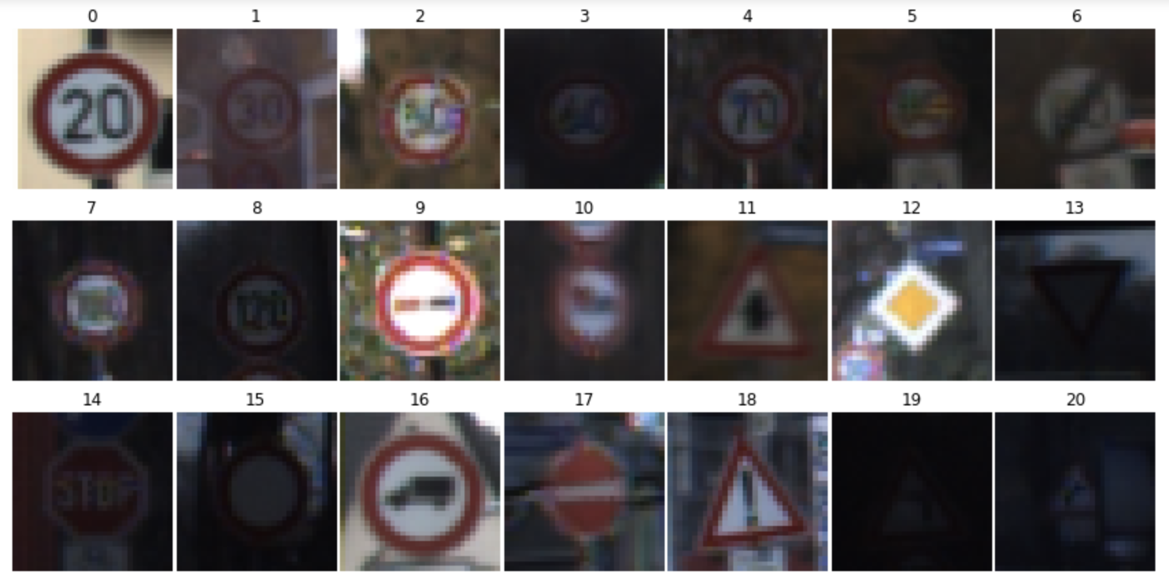
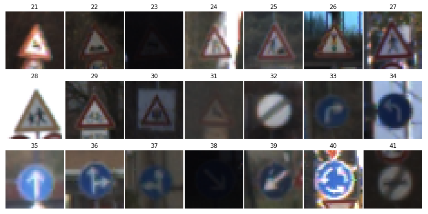
The images below includes a preview of the dataset from class 0 - 41. Their corresponding sign name can be found in mapping
Design and Test Model Architecture
1. Image preprocessing and data augmentation
Three preprocess techniques are used to preprocess image data: gray scaling, normalize pixel value so that every pixel preserves values from [-1, 1] and Lastly standardizing.
Gary scaling the images is a crutial part to simplify training process but eliminating the 3 channels complication at input phase. This tecnique is effective because after previewing the data set, all classes have distinct shapes which means they don't need to be uniquely identified by color. Thus gray scaling the training data set will not sacrifies training accuracy.
Normalization is used so that the input pixel values have similar size, preventing bigger (closer to 255) values being treated with high priority compared to lighter color pixels (closer to 0) thus introducing biases during training.
standadizing techniques are used to normalized input pixel values of every image to have 0 mean because weight decay and Bayesian estimation (not used here but broadly used in machine learning field) can be done more conveniently with standardized inputs.
The above three steps are performed on a testing image as shown below:
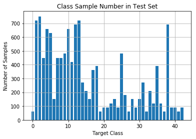
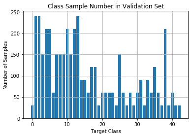
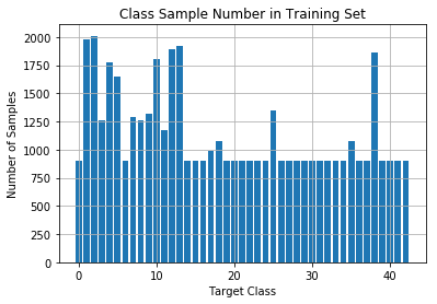
However, another issue of the dataset is big variance between the number of training images among all classes as we see before. To prevent such difference introducing biases during training, data augmentation techniques are used to generate "fake" data from existing training data. To do this, four techniques are used: flip left and right, flip up and down, rotate 90 degrees and zoom in by a factor of 1.5. At first, the mean number of data set if calculated (eg. training set has a mean number of data of 900 images/class). Then all classes with less images are augmented until they have at least 900 images utilizing the above 4 techniques. The final training, valid and test data are as follows.
Notice that the valid and test set is the same as before. Augmenting the valid and test dataset will change the evaluation metrics, and results in different testing conditions and accuracy evaluation compared to other researchers using the same validation and test set
2. Model Architecture
My final model consisted of the following layers:
| Layer | Description |
|---|---|
| Input | 32x32x1 Gray Scled, Normalized and Standardized images |
| Convolution 5x5x1x8 | 1x1 stride, VALID padding, outputs 28x28x8 |
| RELU | |
| Max pooling (conv1) | 2x2 stride, outputs 14x14x8 |
| Convolution 5x5x8x16 | 1x1 stride, VALID padding, outputs 10x10x16 |
| RELU | |
| Max pooling (conv2) | 2x2 stride, outputs 5x5x16 |
| Convolution 4x4x16x300 | 1x1 stride, VALID padding, outputs 2x2x300 |
| RELU | |
| Max pooling (conv3) | 2x2 stride, outputs 1x1x300 |
| Concatenate (conv2 + conv3) | 5x5x16 + 1x1x300 = 1x700 |
| Dropout | Keep probability: 0.5 |
| Fully connected | Weight 700x400, output 1x400 |
| RELU | |
| Fully connected | Weight 400x200, output 1x200 |
| RELU | |
| Fully connected | Weight 200x84, output 1x84 |
| RELU | |
| Fully connected | Weight 84x43, output 1x43 |
| RELU | |
| Softmax |
3. Describe how you trained your model. The discussion can include the type of optimizer, the batch size, number of epochs and any hyperparameters such as learning rate.
The model is trained on NVIDIA 1070 with approximately 5 sec. per EPOCH. The batch size uses 100 images per batch, trained for 30 EPOCHS, learning rate of 0.0009 and keep probability in dropout layer of 0.5.
4. Training result and model tuning
The model achieved final validation accuracy of 95.1% after 30 EPOCHS and 93.1% accuracy in test set. The model adpted the idea from Multiscale Neural Network which achieved 99.17% accuracy in German Traffic Sign classification challenge.
The model tuning process consists of the following steps:
- First model uses LeNet but increased depth of convolutional layer.
- By increasing the convolutional layer depth, more features are expected to be extracted.
- The initial model is being evaluated on "augmented validation and testing dataset" which later proves to be wrong when comparing results with others in the community using the original validation and test set. The augmented validation and test set uses the same techniques used to augment training dataset.
- After discarding the augmented validation and training dataset, the reported accuracy has increased from 85% to 93% with the same architecture as LeNet but deeper convolutional layer.
- By mimicing the architecture used in Multiscale Convolutional Neural Network, 2nd convolutional layer and 3rd convolutional layers are concatenated and further fed into fully connected layers.
- This approch helps propogate the earlier extracted features from 2nd layer being considering together with "higher level feature" extracted from 3rd layer be fed into fully connected layer and takes a part in the final classification.
- This model however experienced with overfitting with almost 97% accuracy in validation set but 92% accuracy in test set.
- Dropout layer with parameter keeping probability of 0.5 is used to prevent overfitting.
- The model no longer has overfitting problem.
- Tuning learning rate higher than 0.001 produces worse model, adjusting the learning rate to 0.0009 results in a better model which is the final model used in this project.
Test a Model on New Images
1. Test on data outside testing dataset
The new images used for testing are shown as below:

These images has much higher qualities even if being resized to 32x32. They should be easy for the model to classify.
2. Test results of new images
Here are the results of the prediction:
| Image | Prediction |
|---|---|
| 100 km/h speed limit | No passing of vehicles over 3.5 |
| Ahead Only | Ahead Only |
| General Caution | General Caution |
| Stop | Stop |
| 70 km/h speed limit | 70 km/h speed limit |
The model was able to correctly classify 4 of the 5 traffic signs, which gives an accuracy of 80%. The test accuracy is 93.1%.
The reasons for such decrease in accuracy are as follows:
- Model too complicated.
- Training set too small.
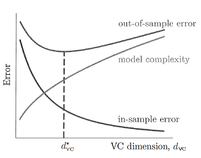
A more complicated model means high vc dimension. In the context of neural networks, deeper convolutional layers or more hidden layers both causes the model to be more complicated thus results in higher vc dimension. As result, more complicated model can easily fit training set more accurately (decrease in-sample error Ein) but losses model generalization skill at the same time. This effect can be observed when testing the model in out-sample test cases.
As shown in the below equations, increasing the number of training images can decrease the gap between in-sample error and out-sample error, which is another method to increase the out-sample error.
Applying only the first method (decrease model complexity) until the model reaches dvc* can produce the minimum out-sample error although in-sample error has a slightly increase. This method is effective because the ultimate goal of training a neural network is to achieve low out-sample error rather than in-sample error (overfitting).
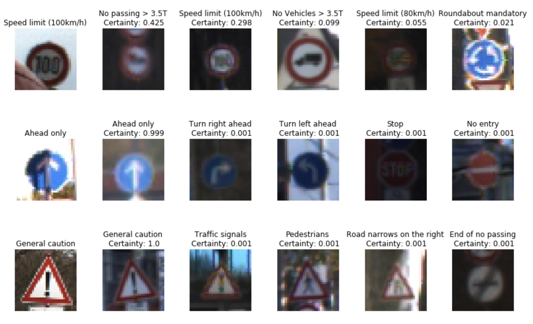
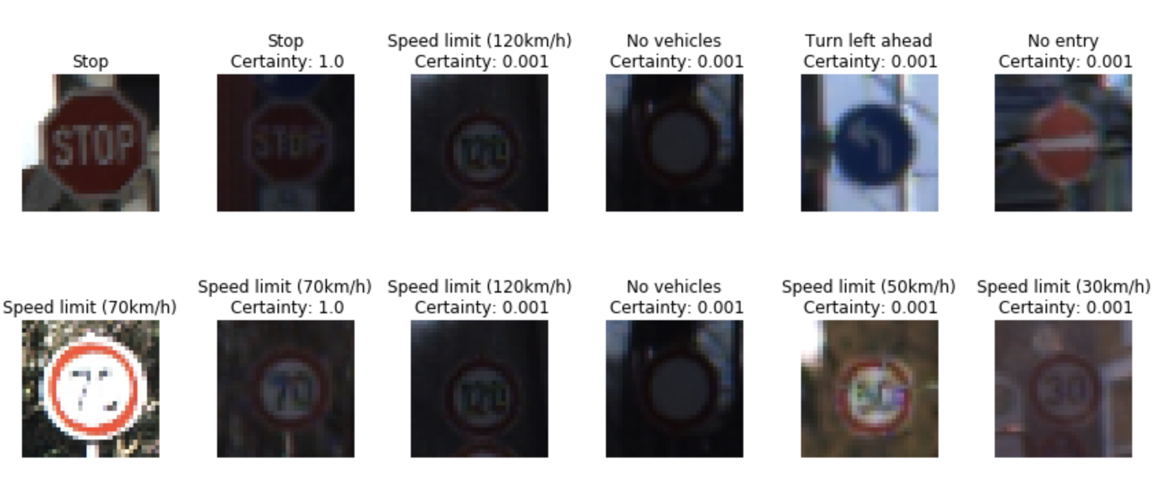
3. Computing the certainty of prediction using Softmax probability to compute centainty from score.
The code for making predictions on my final model is located in the 14th cell of the Ipython notebook. The results are shown as follows:
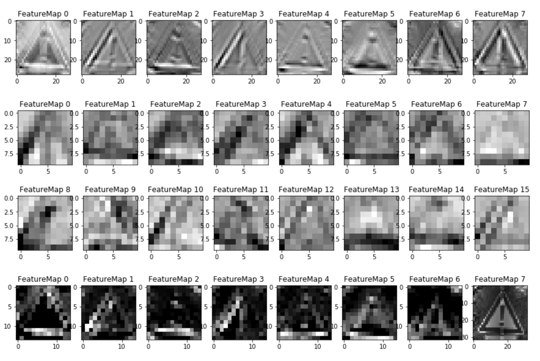
Visualizing the Neural Network
1. Visualization of the Neual Network internal layers
As shwon in the above images, the neural network utilizing the edges and intensity of pixels in the earlier layers and later combine all low level features to produce higher level feature which looks similar to the actual input image.
