Tristanovsk / grs

Atmospheric correction processor for high spatial resolution multispectral satellite images

GRS algorithm package

GRS (Glint Removal for Sentinel-2-like sensors)

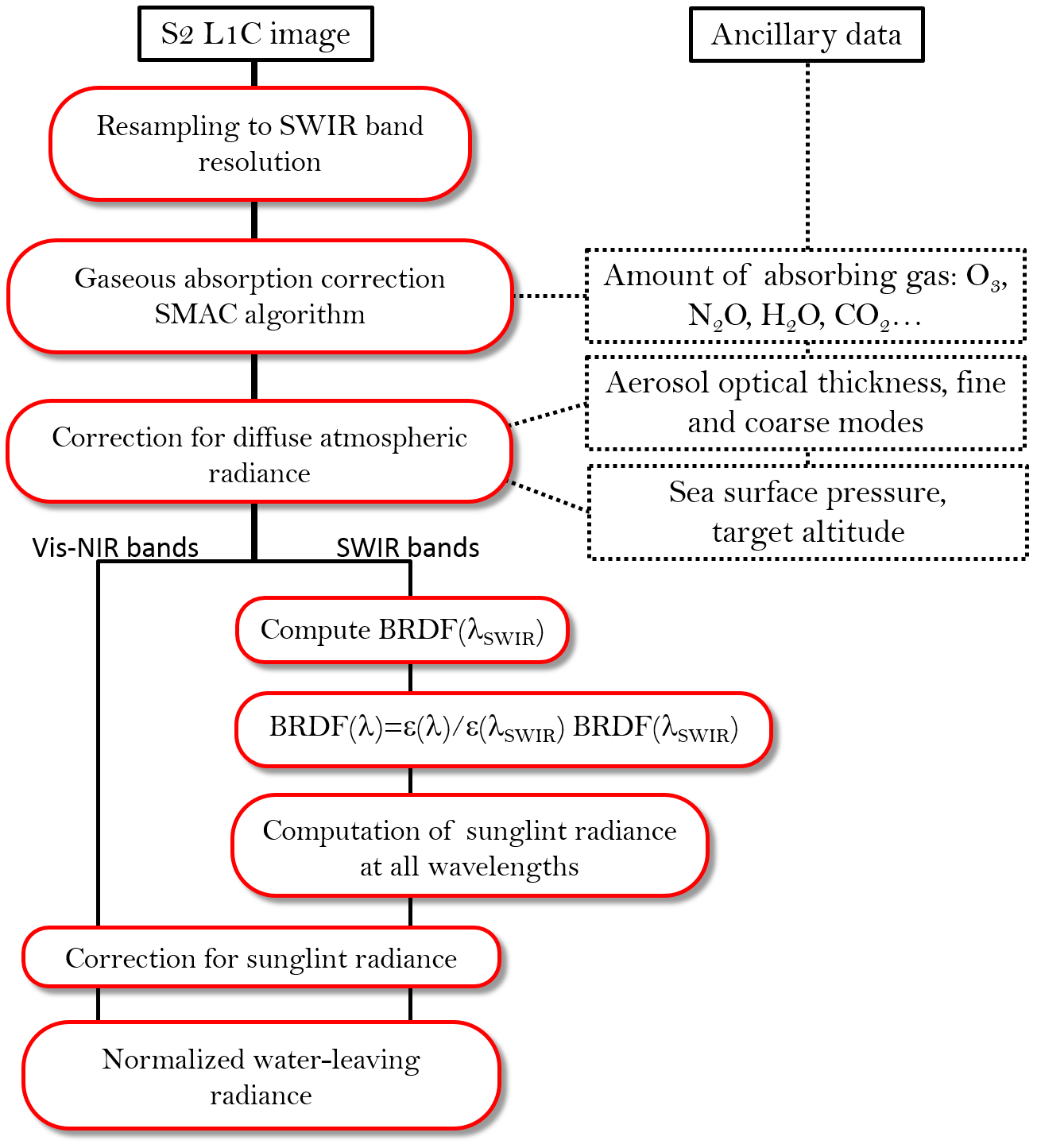
The GRS (Glint Removal for Sentinel-2) algorithm Harmel et al., 2018 was specifically developed to handle and correct for the direct sunlight reflected by the water surface and potentially reaching the sensor (i.e., sunglint signal) of Sentinel-2-like mission, that is nadir or near-nadir viewing sensor with SWIR bands. The GRS processor consists of three main modules to correct for (i) gaseous absorption, (ii) diffuse light from sky and its reflection by the air-water interface and (iii) the sunglint signal in order to retrieve the water-leaving signal at the water surface level.

First, the gaseous absorption (mainly CO2, H2O and O3) correction is performed with the SMAC software (Rahman & Dedieu, 1994) based on parameterizations of the gas transmittances from full radiative transfer computations using 6S (Kotchenova et al., 2006). Atmospheric pressure and gas concentrations are retrieved from bilinear interpolation within the grid of the Copernicus Atmosphere Monitoring Service dataset (CAMS). Then, spectral radiances are corrected for the diffuse sky light and its reflection on the air-water interface. For each pixel, the diffuse radiance component is reconstructed for the given viewing geometry (i.e., sensor and Sun viewing angles and relative azimuth) from pre-computed look-up tables (LUT). The Rayleigh optical thickness is rescaled based on the actual pressure at the scene level to take into account the effects of the altitude on the scattering properties of the atmosphere. Those LUTs were generated based on the radiative transfer model OSOAA (Chami et al., 2015) for a typical fine and coarse mode aerosol models, encompassing weakly absorbing ones (Levy et al., 2009), and including the specific spectral response of the sensor bands. The atmosphere plus surface diffuse signal $L_{sky}$ is obtained considering a bimodal aerosol model (Wang & Gordon, 1994) as follows:

where $L_{sky}^{fine}$ and $L_{sky}^{coarse}$are the radiances for the fine and coarse aerosol modes, respectively, for the aerosol optical thickness $\tau _a$; $\gamma$ is the mixing coefficient corresponding to the relative amount of each mode in the atmosphere. Note that $\tau _a$ is obtained from the CAMS dataset (Benedetti et al., 2008; Morcrette et al., 2009) and $\gamma$ is retrieved from non-linear fitting including the LUT aerosol parameters with the spectral values of $\tau _a$ provided by CAMS.

Regarding the sunglint correction, the main principle is to estimate the bidirectional reflectance distribution function (BRDF) of the rough air-water interface from the SWIR bands (i.e., ~1610 and ~2200 nm). The sunglint signal obtained in the SWIR is then extrapolated toward the NIR and visible bands. Estimation of the sunglint radiance is based on the fact that water body is virtually totally absorbing; water absorption coefficient in the SWIR is several orders of magnitude greater than that in the NIR. Once corrected for atmosphere diffuse radiance, the remaining radiance in the SWIR is interpreted as the pure surface component of the signal and then translated into BRDF. This BRDF in the SWIR is extrapolated to the other bands considering the spectral variation of the refractive index of water and its important consequences onto the spectral sunglint signal (see Harmel et al., 2018 for details). The sunglint radiation is calculated for each pixel, for each band, considering the estimated BRDF, atmosphere direct transmittance and the extraterrestrial sun radiance reaching the atmosphere, and the water-leaving radiance is then corrected by removing this value.

The water-leaving component at the water surface level is eventually obtained after division by the total transmittance (i.e., diffuse + total transmittances) calculated for the bimodal aerosol model from the LUT. The version used here accounts for the spectral response of each band of Sentinel-2 A and B as well as Landsat-8 and it is based on the CAMS aerosol data for the spectral value of $\tau _a$.

Getting Started

These instructions will get you a copy of the project up and running on your local machine for development and testing purposes. See deployment for notes on how to deploy the project on a live system.

Prerequisites

Register and ask for a key to use ECMWF API

Download and install the SNAP software. Configure the SNAP-python interface and link the obtained snappy folder to your python site-packages as esasnappy. For example:

ln -s /FULL_PATH/.snap/snap-python/snappy /PATH_TO_LIB_PYTHON/lib/python3.6/site-packages/esasnappy

Compilers such gcc and gfortran are needed to install the package.

Bindings are made based on F2PY. Please update the version of F2PY accordingly to your python version in Makefile; for instance:

export F2PY=f2py3.6

Compile all C and fortran files into shared libraries:

make

Generate the config.py file:

• In the ./grs/grs folder, copy config_local.py to config.py.

• Then, edit config.py according to your folders tree and path to your grs installation folder.

Load the data folder grsdata containing the auxiliary data and look-up tables (LUT) from here, unzip and edit the variable data_root with the full path of your grsdata folder.

Installing

To install the package:

python setup.py install

or

python setup.py install --user

If the installation is successful, you should have:

$ grs
Usage:
  grs <input_file> [--sensor <sensor>] [-o <ofile>] [--odir <odir>] [--shape <shp>] [--wkt <wktfile>]   [--longlat <longmax,longmin,latmax,latmin> ]    [--altitude=alt] [--dem] [--aerosol=DB] [--aeronet=<afile>]    [--aot550=aot] [--angstrom=ang] [--output param]   [--resolution=res] [--levname <lev>] [--no_clobber] [--memory_safe] [--unzip]
  grs -h | --help
  grs -v | --version

On the PBS cluster : installing from sources with conda on the cluster CNES

Create the conda environment using the definition file available in the conda folder :

conda env create -f conda/grs_conda_3.6.yml -p /work/scratch/$user/grs_py3.6

The option -p set the directory where the conda environment will be installed

To install the package grs in conda :

source conda/conda_grs.sh -ci

To launch GRS on a pbs node :

qsub launch_grs_exemple.pbs

Running the tests

From terminal:

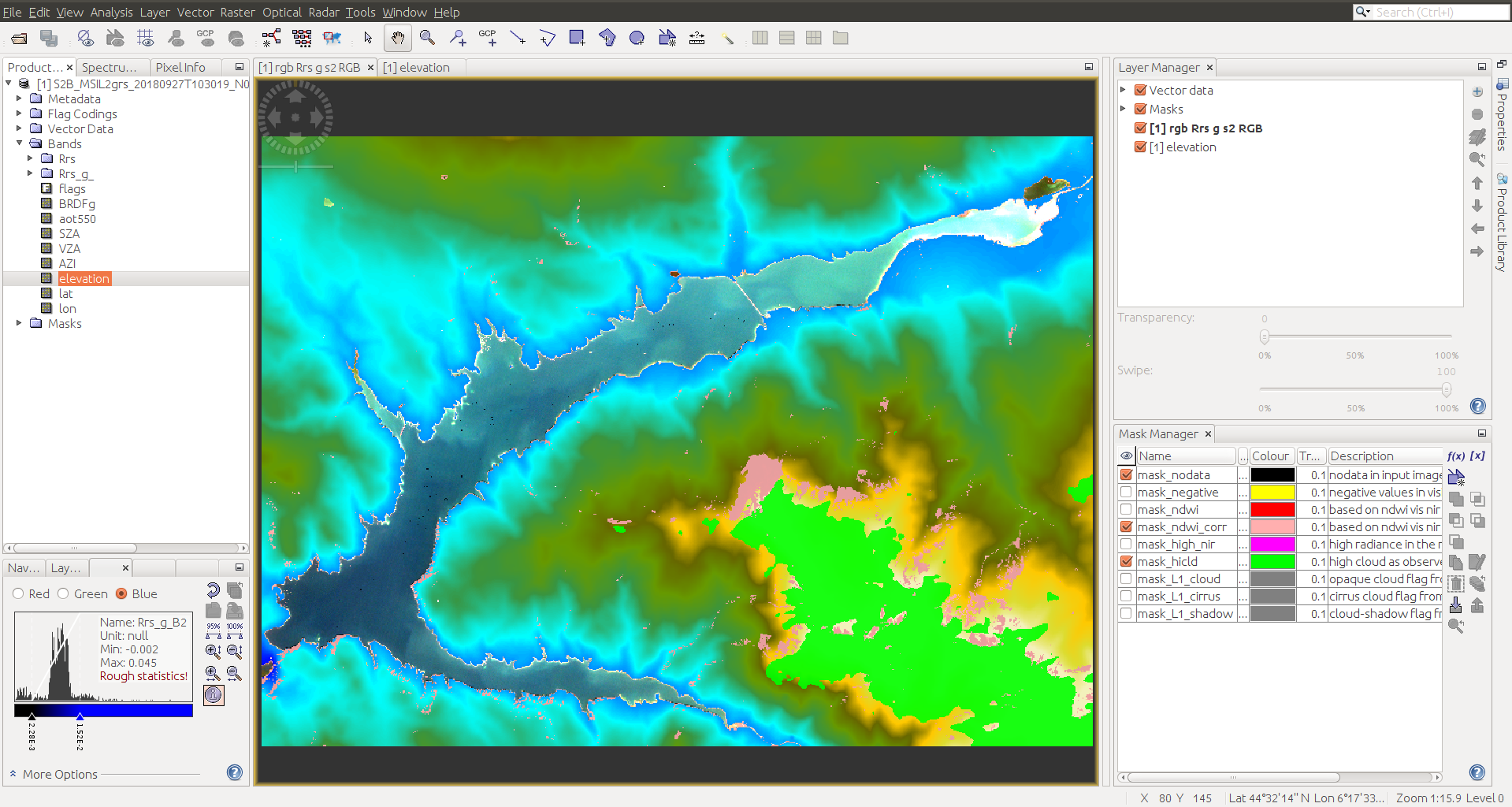
grs test/data/S2B_MSIL1C_20180927T103019_N0206_R108_T31TGK_20180927T143835.SAFE --shape test/data/shape/SPO04.shp --odir test/results/ --aerosol cams_forecast --dem --resolution 20

You should get something like:

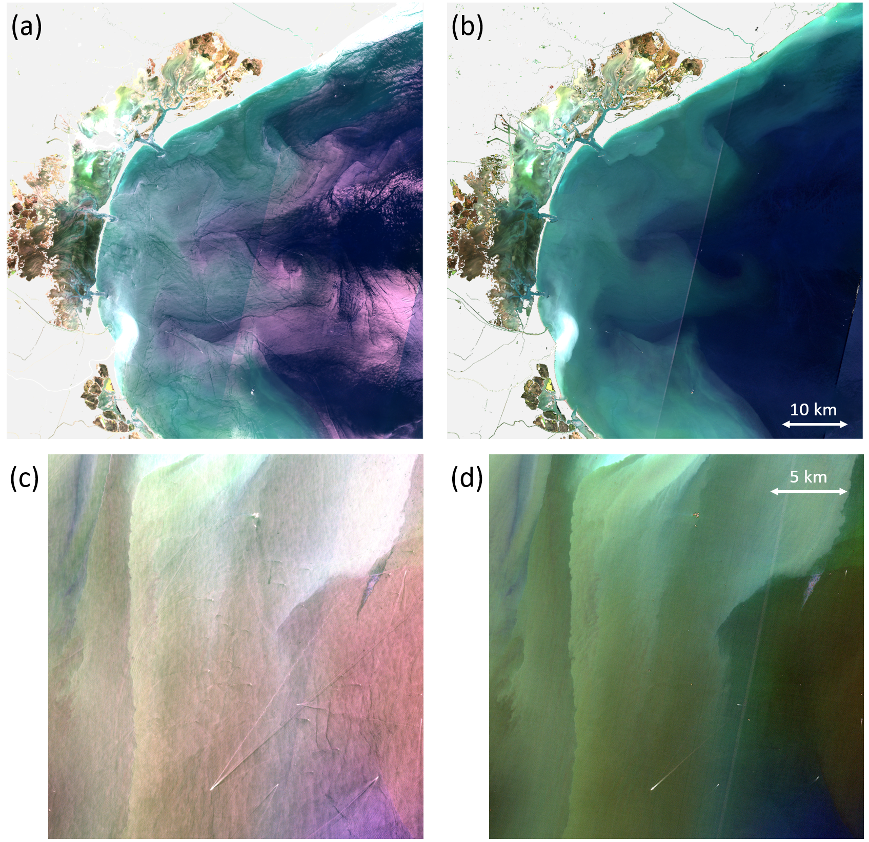
Another examples of output images before (1st column) and after (2nd column) sunglint correction:

Deployment

See examples in exe.

Contributing

Please contact authors for details on our code of conduct, and the process for submitting pull requests to us.

Authors

• Tristan Harmel - Initial work - contact

See also the list of contributors who participated in this project.

License

This project is licensed under the MIT License - see the LICENSE.md file for details

Acknowledgments

• The Step forum and Marco Peters are acknowledged for their useful help to process Sentinel-2 data with the snappy API.
• The authors are very grateful to Olivier Hagolle for providing open source codes to perform gaseous absorption correction and massive Sentinel-2 data download.