Triang-jyed-driung / Adaptive-BVP

Implementation of the "A fast adaptive numerical method for stiff two-point boundary value problems" by June-Yub Lee and Leslie Greengard

Adaptive-BVP

Course Project, Numerical Analysis, Spring 2023

基于Python的二阶常微分方程两点边值问题自适应求解器（清华大学求真书院2023年春季数值分析课程大作业）

Implementation of the A fast adaptive numerical method for stiff two-point boundary value problems by June-Yub Lee and Leslie Greengard. Below is a full report.

Contents

• Introduction
• Linear solver
• Nonlinear Solver
• Examples
• Adaptivity
• FAQ
• Advantages and defects
• Conclusion

Introduction

This project contains:

• A Python program named BVPSolver.py, which contains two solvers.
• A test program named test_all.py, which runs all examples in sequential order. See below for all 6 examples.
• A specification/report in Markdown format (this file).

To use the solvers, Add this line to the top of your code:

import BVPsolver

or

from BVPsolver import LinearBVPSolver, NewtonNonlinearSolver

This Python program contains 2 main functions, LinearBVPSolver for linear BVPs, and NewtonNonlinearSolver for nonlinear BVPs.

This project is solely for academic purpose and is NOT ready for any serious scientific computing or for production use.

Tested with:

• Windows 10
• Python 3.11.2
• Numpy 1.24.2
• Matplotlib 3.7.1

Other versions are likely to work as well.

Linear solver

To solve linear equations, please use LinearBVPSolver function. The function LinearBVPSolver has the following parameters:

def LinearBVPSolver(p, q, f, a, c, zetal0, zetal1, gammal, zetar0, zetar1, gammar,
    C=4.0, TOL=1e-8, iters=40, eval_points=32, force_double=False):

This function aims to solve the following ordinary differential equation: $$u''(x) + p(x) u'(x) + q(x) u(x) = f(x)$$ with respect to boundary conditions: $$\zeta_{l0} u(a) + \zeta_{l1} u'(a) = \gamma_l$$ and $$\zeta_{r0} u(c) + \zeta_{r1} u'(c) = \gamma_r$$.

• p: A function defined on $[a,c]$ and returns a float number.
• q: A function defined on $[a,c]$ and returns a float number.
• f: A function defined on $[a,c]$ and returns a float number.
• a: A float number for the left boundary of the interval.
• c: A float number for the right boundary of the interval.
• zetal0, zetal1, gammal, zetar0, zetar1, gammar: float numbers determining the boundary conditions $\zeta_{l0} u(a) + \zeta_{l1} u'(a) = \gamma_l$ and $\zeta_{r0} u(c) + \zeta_{r1} u'(c) = \gamma_r$.
• C: A float number with the same meaning described in the article. Default to 4.0.
• TOL: Error tolerance, default to 1e-8.
• iters: Number of allowed refinement iterations to solve the equation to the given error tolerance. Default to 40.
• eval_points: This program calculates the function values at eval_points random points on $[a,c]$ to estimate the error. Default to 32.
• force_double: The algorithm in the article contains one last doubling step, splitting every subinterval node into two to ensure that error stays within TOL. In my experiments, this step is usually unnecessary and doubles the execution time. Default to False. Switch it to True to force the same behavior described in the article.

This function returns a class LinearBVPSolver.Node that is directly callable. If you have already set u = LinearBVPSolver(...), then you can:

• Access function value at x, i.e., $u(x)$, by direclty calling u(x).
• Access function derivative at x, i.e., $u'(x)$, by calling u(x, deriv=True). The function value or derivative at x is computed by Chebyshev interpolation, which is more accurate than linear or spline interpolation.

Example usage:

from scipy.special import jv
from matplotlib import pyplot as plt
import numpy as np
from BVPSolver import LinearBVPSolver
u = LinearBVPSolver(
    lambda x: 1/x,
    lambda x: 1-(100/x)**2,
    lambda x: 0,
    0, 600,
    1,0,0,
    1,0,1,
    TOL=5e-10,
)
xs = np.linspace(0, 600, 600)
plt.plot(xs, [u(xi) for xi in xs])
plt.title("Bessel 100 on [0,600]")
plt.show()

Nonlinear solver

The function NewtonNonlinearSolver has the following parameters:

def NewtonNonlinearSolver(
    f, f_2, f_3, a, c, zetal0, zetal1, gammal, zetar0, zetar1, gammar,
    initial=None, C=4.0, TOL=1e-6, iters=10, eval_points=32, force_double=False,
):

This function aims to solve the following ordinary differential equation: $$u''(x) = f(x, u, u')$$ with respect to boundary conditions: $$\zeta_{l0} u(a) + \zeta_{l1} u'(a) = \gamma_l$$ and $$\zeta_{r0} u(c) + \zeta_{r1} u'(c) = \gamma_r$$.

• f: A function that accepts 3 float numbers (namely x, u, du where du is $u'(x)$) and returns a float number.
• f_2: Partial derivative of f with respect to the second parameter, which is $\partial_2 f$. It also accepts 3 float numbers (namely x, u, du where du is $u'(x)$) and returns a float number.
• f_3: Partial derivative of f with respect to the third parameter, which is $\partial_3 f$. It also accepts 3 float numbers (namely x, u, du where du is $u'(x)$) and returns a float number.
• a: Same as above
• c: Same as above
• zetal0, zetal1, gammal, zetar0, zetar1, gammar: Same as above
• initial: Provide an initial guess for the Newton's method. Default to None. If you want to provide an initial guess, set initial=(u0,du0) where u0 is the initial guess function and du0 is its derivative. If not specified, the program automatically chooses an initial guess, which coincides with the $u_i$ described in the article.
• C: Same as above
• TOL: Error tolerance, default to 1e-6.
• iters: Maximum number of Newton iterations to solve the equation. Default to 10.
• eval_points: Same as above
• force_double: Same as above

This function also returns a class LinearBVPSolver.Node that is callable as a function. See above for details.

The formula of Newton's iteration is not explicitly specified in the article. Here is the formula:

Let $u_{n+1}(x)$ solve

$$u''_{n+1} -\partial_3 f(x, u_n, u'_n) u'_{n+1} -\partial_2 f(x, u_n, u'_n) u_{n+1}=f(x, u_n, u'_n) -\partial_3 f(x, u_n, u'_n) u'_n -\partial_2 f(x, u_n, u'_n) u_n$$

The above iteration process is repeated until the solution reached within desired error tolerance.

Try this example, or see the example 4 below for details:

from matplotlib import pyplot as plt
import numpy as np
from BVPSolver import NewtonNonlinearSolver
r = NewtonNonlinearSolver(
    lambda x, u, du: 2*u*du,
    lambda x, u, du: 2*du,
    lambda x, u, du: 2*u,
    -np.pi/4, np.pi/4,
    1,0,-1,
    1,0,1,
    initial=(lambda x: x**2, lambda x: 2*x),
    TOL=1e-13
)
xs = np.linspace(-np.pi/4, np.pi/4, 100)
plt.plot(xs, [r(xi) for xi in xs])
plt.title("u''=2uu', u=tanx")
plt.show()

Examples

The program is tested across six different examples. Run python test_all.py to sequentially test all the examples below.

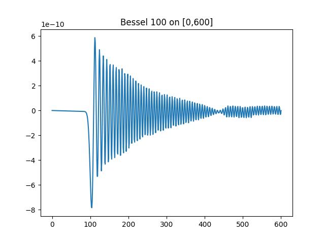
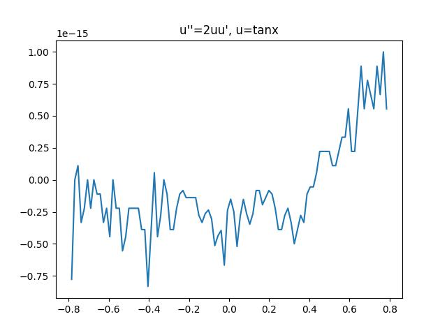
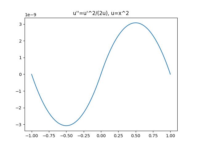
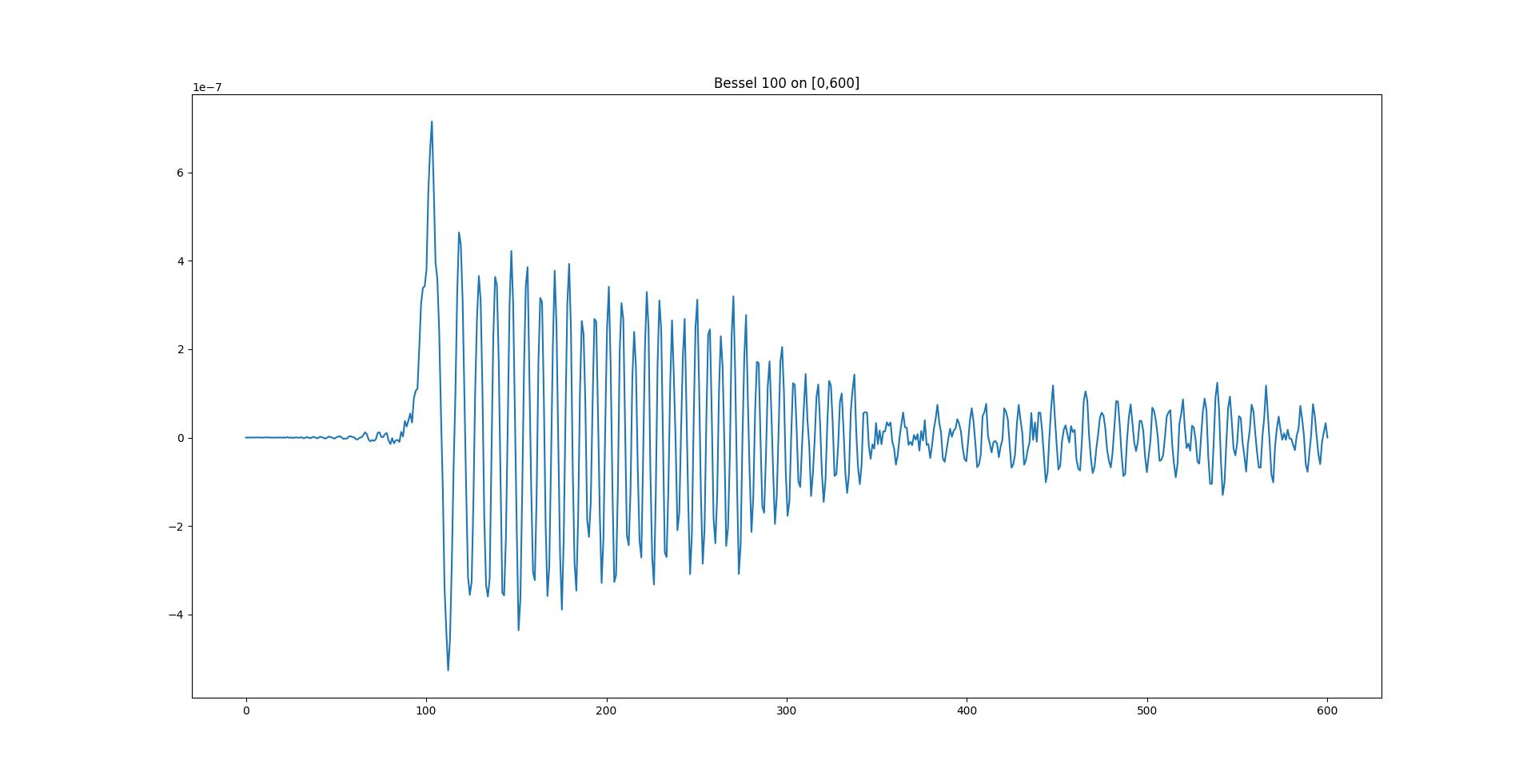
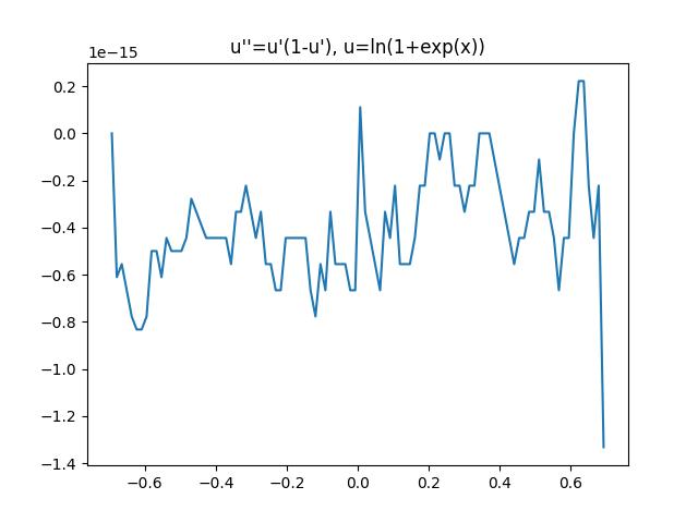
Note: All following 6 plots plot the difference of the computed solution and the real sulution.

In all these experiments, we set K = 16, namely 16 chebyshev nodes.

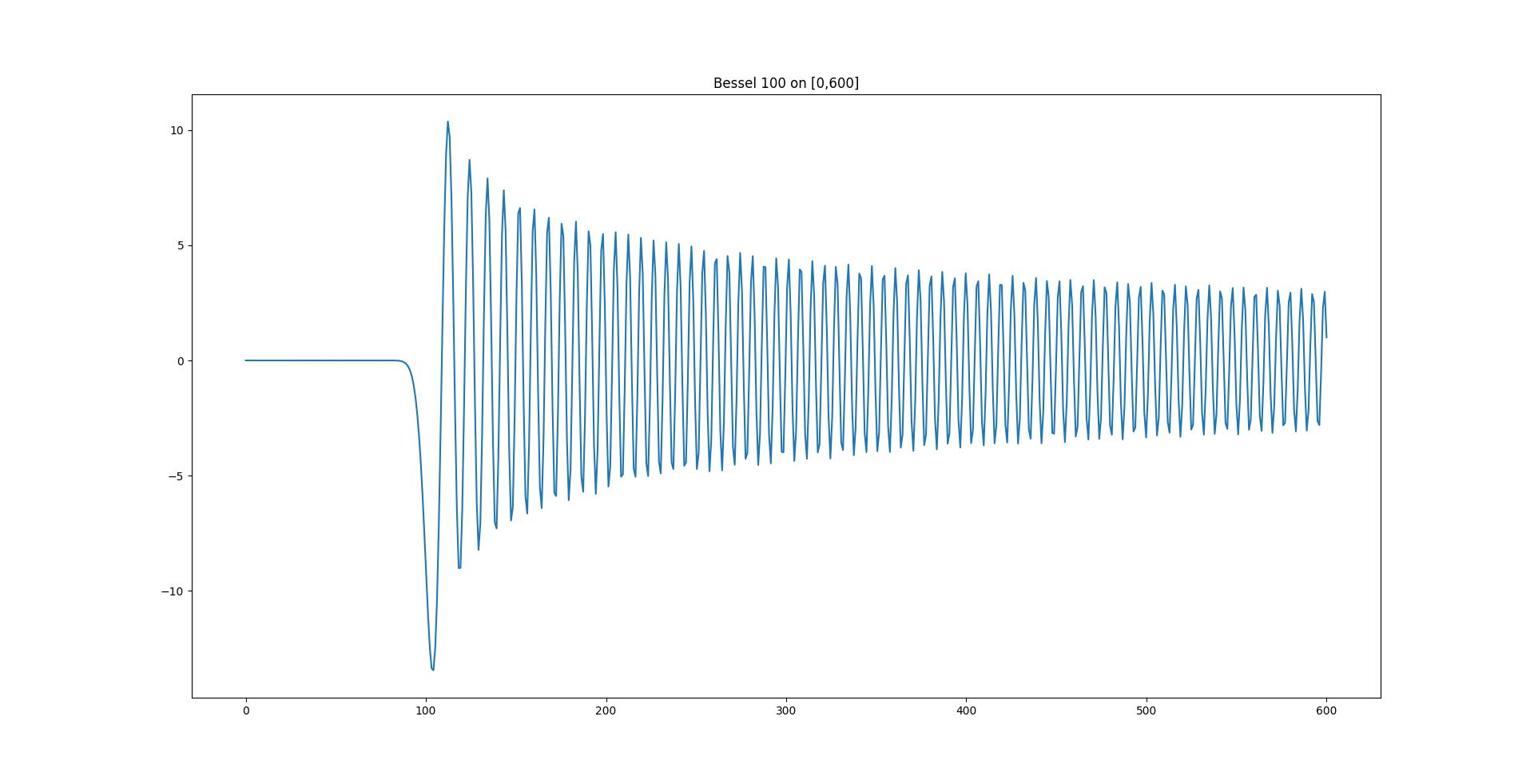
1. Bessel J function example, from the article:

$$u''+\frac{u'}{x} + \frac{x^2-100^2}{x^2} u = 0 \text{ on } [0,600], \quad u(0)=0, \ \ u(600)=1$$

The solution is:

$$u(x) = \frac{J_{100}(x)} {J_{100}(600)}$$

The program runs 18 iterations with 204 subintervals, the time spent is 0.725s.

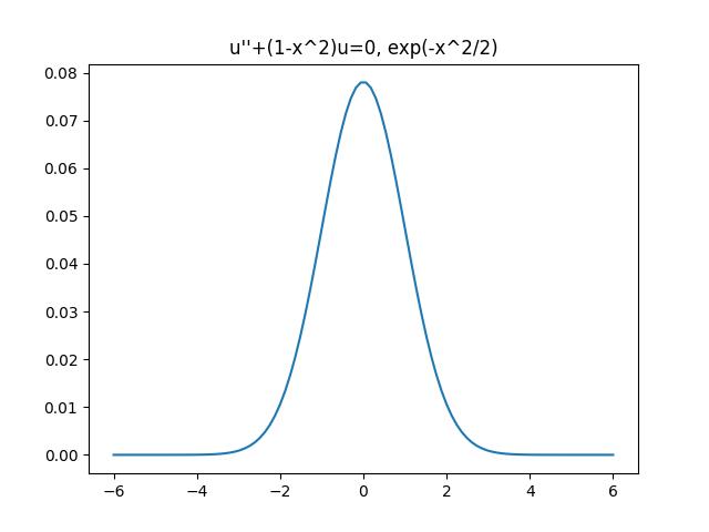
2. "Base state of quantum harmonic oscillator"

$$u''+ (1-x^2) u = 0 \text{ on } [-6,6], \quad u(-6)=u(6)=e^{-18}$$

The solution is:

$$u(x) = \exp \left( - \frac{x^2}{2} \right)$$

This is a ill-conditioned problem. This solution fails to converge because $e^{-18}$ is too small compared to $u(0) = 1$ in the true solution, so small roundoff pertubations lead to significant errors. But fortunately, the shape of the solution is correct.

Note: This sover is programmed to automatically exit when there are more than 1024 intervals. This is partly because that systems with a large number of intervals require significantly longer time to solve.

The solver runs 13 iterations with 1405 subintervals, and forced to exit because there are more than 1024 intervals. The time spent is 2.289s.

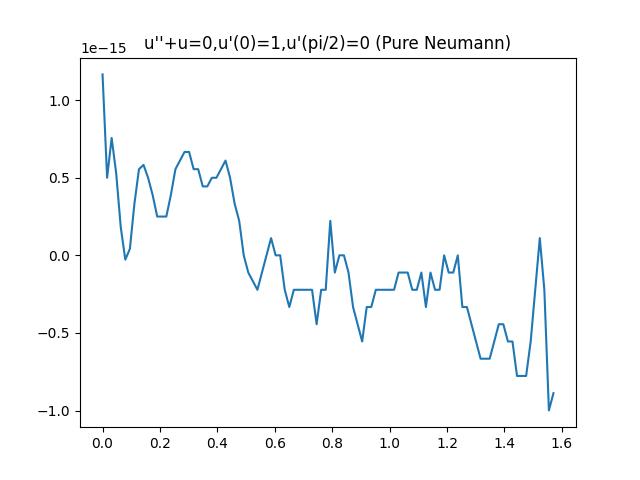
3. Neumann condition test

$$u''+ u = 0 \text{ on } [0,\pi/2], \quad u'(0)=1,u'(\pi/2)=0$$

The solution is:

$$u(x) = \sin(x)$$

This is a simple example, yet it failed during my debugging process. Now it's fixed and the solution achieves machine precision.

The solver runs 2 iterations with 2 subintervals. The time spent is 0.005s, and achieves machine precision.

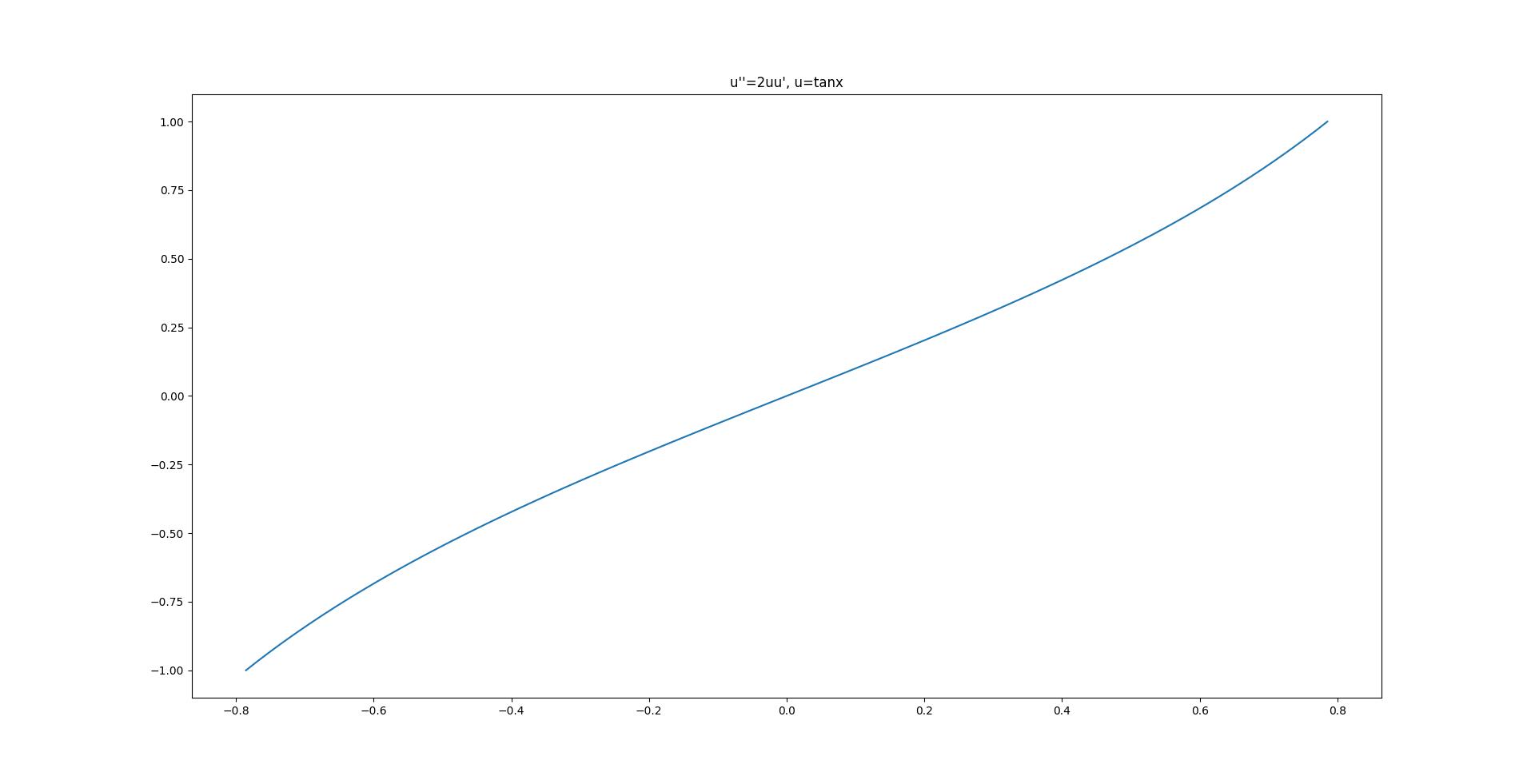
4. The tangent function

$$u''-2uu'=0 \text{ on } \left[-\frac{\pi}{4},\frac{\pi}{4}\right], \quad u\left(\frac{\pi}{4}\right) = -u\left(-\frac{\pi}{4}\right) = 1$$

The initial guess: $u_0(x) = x^2$, which is not a good guess. The solution is:

$$u(x) = \tan(x)$$

This is a simple example to test the Newton solver. It quickly achieves machine precision.

The solver runs 6 iterations with 6 subintervals. The time spent is 0.280s, and achieves machine precision.

5. A homogeneous nonlinear example

$$u'' = \frac{u'^2}{2u} \text{ on } [-1,1], \quad u(-1)=u(1)=1$$

The initial guess: $u_0(x) = x$, which makes up a singularity for $\frac{u'^2}{2u}$ at $x=0$. The solution is:

$$u(x) = x^2$$

This example is interesting because although the final solution converges, $\frac{u'^2}{2u}$ shows a singularity at $u=0$. The solver handles it correctly, but failed to reach machine precision.

The Newton solver runs 6 iterations. The time spent is 2.456s. The first 2 Newton iterations are particularly long due to a singularity.

6. Logistic

$$u'' = u'(1-u') \text{ on } [-\ln(2),\ln(2)], \quad u'(-1)=\frac 1 3,\ \ u(1) = \ln(3)$$

The solution is:

$$u(x) = \ln(1+exp(x))$$

This is a classic example, to test a mixed boundary condition.

The Newton solver runs 4 iterations on at most 2 intervals. The time spent is 0.046s, and the solution achieved machine precision.

Adaptivity

Ablation studies are conducted to demonstrate adaptivity. Here, we tested the same example as example 1 (Bessel $J_{100}$). We use one single interval with 2048 Chebyshev points, without adaptivity. The results:

The results showed that the difference is about $1e-7$, which is a much higher error than the adaptive version. Hence, adaptivity is important.

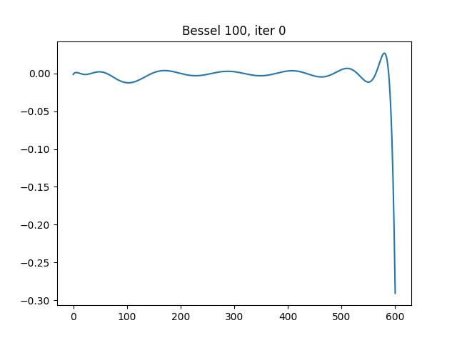
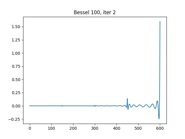
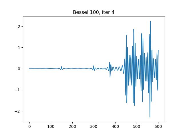
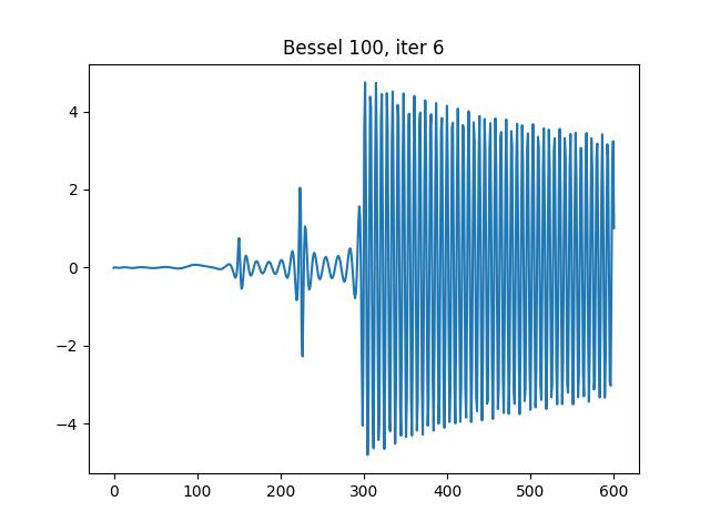
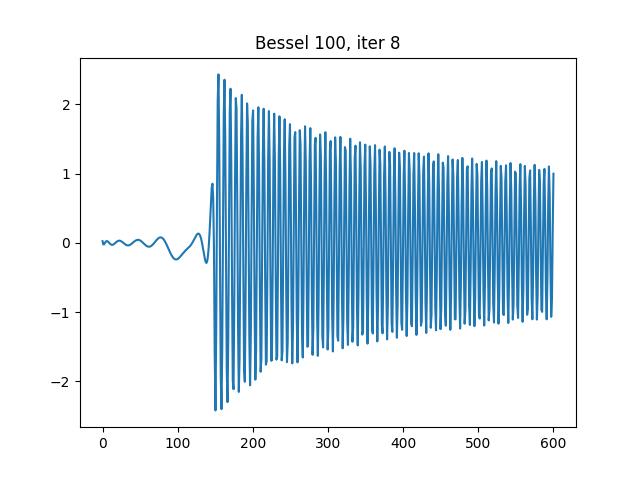
Auto-adaptivity is also studied. the experiments with intermediate results are presented as follows:

Iteration 0, 1 interval:

Iteration 2, 4 intervals:

Iteration 4, 8 intervals:

Iteration 6, 19 intervals:

Iteration 8, 35 intervals:

Iteration 10, 48 intervals:

Iteration 17, 204 intervals, the final result, with error about $1e-10$:

FAQ

Q: What can be said about the (rank) structure of the matrix A in the computation?

A: There is no definitive answer. In most cases, A is a full rank matrix, becaude almost all square matrices are full-rank. but the cases where A is degenerate are encountered. Therefore, it is generally better to use a generalized solver to solve the least-square or least-norm problem that handles degenerate case. For example, np.linalg.lstsq is better than np.linalg.solve.

Q: Newton's method (in its pristine form) is very sensitive to the choice of initial guess. Do you have a method to overcome this difficulty for your two-point BVP solver?

A: We can make multiple initial guesses. However, I don't know how to solve it entirely in a black-box fashion.

Q: Chap 2.4 (Theorem 2.13 and 2.14) in Starr and Rokhlin discusses the case with degenerate boundary conditions. They presented one relevant example (Example 5) with degenerate BC. In that example, they constructed a transform manually, which is a bit unsatisfying. Can you deal with degenerate BCs in a black-box fashion?

A: Degenerate boundary condition is heavily related to Sturm-Liouville problems. The spectrum of Sturm-Liouville problems is discrete, so only at certain specific points does the BVP with degenerate boundary conditions possess a nontrivial solution. For example, $u''=-u$, $u(0)=u(l)=0$. When $l$ is a multiple of $\pi$, then the equation has infinitely many solutions, but otherwise, it has only the zero solution.

Advantages and defects

Advantages

• The solver function returns a class object which contains all the necessary information, including binary tree structure and chebyshev points, and itself is easily callable as a function.
• Chebyshev interpolation enables higher order of accuracy.
• A good solver (numpy.linalg.lstsq) that handles degenerate cases and avoids crashing.

Defects

• Cannot identify unsolvable cases - While numpy.linalg.lstsq handles degenerate cases efficiently, it does not report unsolvable cases explicitly by raising an error. If the equation itself is unsolvable, this program might silently output an approximate "solution". Similarly, it does not explicitly handle cases where there are multiple possible solutions.
• Possible early stop - To improve speed, the final doubling step where all intervals are splitted into halves is disabled by default. This may cause early stops. Also, random sample points are used to evaluate the tolerance TOL, hence it's entirely possible that all random points fall on one side of the interval, ignoring singularity on the other side.
• Slower speed - As a Python program, its speed is intrinsically slower than the same program written in compilable languages, such as C++/C/Fortran.

Conclusion

We have successfully developped the fast adaptive solver for second order two-point BVPs. It yields decent results, finishes in seconds in all tested cases, achieving a precision of at least 1e-8 except extreme cases, and is auto-adaptive.