Lars Snipen
Install the package from CRAN (https://cran.r-project.org/) in the standard way, either by
install.packages("micropan")or by using the Tools - Install Packages… menu in RStudio.
You may also install directly from this GitHub site:
devtools::install_github("larssnip/micropan")If you use this package, please cite this paper.
Let us first have a look at how we can download public genome data. There are many approaches, this is just one of them.
Here is a short video on how to do the following steps.
First, make a folder for this tutorial, and set this as your working directory in R.
Look up the NCBI/Genome database, and click your way to the
browsing of microbes. Here we search for the species
Buchnera aphidicola. This species has small genomes, making the
computations in this tutorial fast. We download the comma-separated
table listing these genomes, and store it with the proper name
Buchnera_aphidicola.csv into a subfolder named rawdata/.
Regardless of how you obtain the genome data, it is strongly recommended
you make a genome table where each row lists all relevant information
about each genome in your pan-genome study. This table typically
contains some name and other information for each genome, and the
genome_id required. The latter is a unique genome identifier
consisting of the text "GID" followed by an integer. Several of the
functions in this package search for this information using the regular
expression "GID[0-9]+", which means you have to follow this exact
pattern.
Let us make a script and read the comma-separated table we downloaded into R and
- Select the columns we find relevant
- Add the
genome_idcolumn - Add a
GenBank_IDcolumn (see below) - Slice only a subset of the genomes, to speed up this tutorial
We will use some tidyverse functions (install the tidyverse
packages) for this. Make a script, and use your micropan tutorial folder
as working directory:
library(tidyverse)
gnm.tbl <- suppressMessages(read_delim("rawdata/Buchnera_aphidicola.csv", delim = ",")) %>%
  select(Name = `#Organism Name`, Strain, Level, GenBank_FTP = `GenBank FTP`) %>%
  mutate(genome_id = str_c("GID", 1:n())) %>%
  mutate(GenBank_ID = str_remove(GenBank_FTP, "^.+/")) %>%
  slice(1:10)
In this case we keep the columns Name, Strain, Level and
GenBank_FTP address for each genome. You may of course add all types
of information about the genomes as columns to this table.
The NCBI/GenBank genome FASTA files are currently stored according to a
system that makes them accessible by using the URL address in the
GenBank_FTP column only. The last term of this address is the name of
the folder in which we find all GenBank data about the corresponding
genome. The files in this folder typically have this as their prefix,
and storing it as a separate column GenBank_ID makes later code
somewhat shorter.
At the time of writing this table contains 76 genomes. To make faster computations in this tutorial, we slice the table down to only the 10 first genomes. You may run with the full table if you like, but this will take (much) longer time.
We are ready to start downloading, and here is some code to do the job.
The genome file names consists of the GenBank_ID and the suffix
_genomic.fna.gz, at least at the time of writing. Note that we also
immediately uncompress the files (using gunzip() from the R.utils
package), since this will be a benefit later.
library(R.utils)
for(i in 1:nrow(gnm.tbl)){
  filename <- str_c(gnm.tbl$GenBank_ID[i], "_genomic.fna.gz")
  download.file(url = file.path(gnm.tbl$GenBank_FTP[i], filename),
                destfile = file.path("rawdata", filename))
  gunzip(file.path("rawdata", filename), overwrite = T)
}
We could also have done this by using the accession numbers in the
columns Replicons and WGS of the downloaded table, and the functions
entrezDownload() and getAccessions() in this R package. They will
download from the Nucleotide database, resulting in uncompressed FASTA
files.
A note on compressed files: Below we make use of the software prodigal
to find genes, and this cannot take compressed fasta files as input. For
reading or writing files in R using readFasta() or writeFasta() you
may very well work with compressed files.
A pan-genome analysis focuses on the coding genes from each genome. Finding these coding genes is a very crucial step for many downstream analyses. Prokaryotic gene finders will usually find most coding genes, but not perfectly. Let us first illustrate this.
We will use the function findGenes() from the microseq package for
this job. This implements the
prodigal gene finding software,
which is very popular. You need to have the software prodigal installed
in order to run this, see the Help page for findGenes().
Let us use as input a ‘genome’ consisting of 1 million basepairs of
uniform random DNA. We make a subfolder tmp/ for storing temporary
files, and put this rubbish ‘genome’ into it
library(microseq)
dir.create("tmp")
set.seed(2020)
tibble(Header = "Random_noise",
       Sequence = str_c(sample(c("A","C","G","T"), size = 1e+6, replace = T), collapse = "")) %>%
  writeFasta(out.file = "tmp/random.fna")
Then we do the gene finding from these data:
gff.tbl <- readFasta("tmp/random.fna") %>% findGenes()The resulting GFF-table lists more than 1000 genes, even if the input is
completely rubbish! It is quite typical of gene finding software tools
that they tend to ‘find genes’ even if there are none. There are many
good reasons for designing them over-sensitive like this, but for
pan-genome studies it is not beneficial. However, this table also has a
column Score given by prodigal
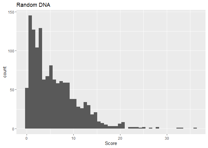
to each of these ‘genes’. A histogram of these scores shows…
fig1 <- ggplot(gff.tbl) +
  geom_histogram(aes(x = Score), bins = 50) +
  labs(title = "Random DNA")
print(fig1)
…that the largest scores are just over 30, and none are above 40. If we use the same procedure on the first real genome
gff.tbl <- readFasta(file.path("rawdata", str_c(gnm.tbl$GenBank_ID[1], "_genomic.fna"))) %>% findGenes()
fig2 <- ggplot(gff.tbl) +
  geom_histogram(aes(x = Score), bins = 50) +
  labs(title = "Real genome")
print(fig2)
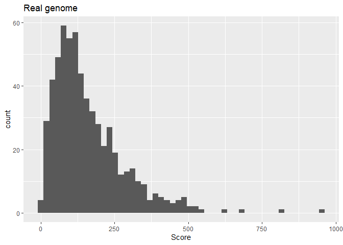
we notice that most genes have scores well above 40, but a few have a very low score, and may be discarded. Such low-scoring gene predictions are likely to be errors, and will affect some of our downstream analyses. These typically end up as cloud genes in the pan-genome, and will affect estimates on pan-genome size and openness severely.
Let us use a cutoff of score 40, to discard the most uncertain gene
predictions. We then extract the coding genes from the genome and
translate them into protein, and store this into the tmp/ folder:
for(i in 1:nrow(gnm.tbl)){
  genome <- readFasta(file.path("rawdata", str_c(gnm.tbl$GenBank_ID[i], "_genomic.fna"))) # for use below
  findGenes(genome) %>%
    filter(Score > 40) %>%
    gff2fasta(genome) %>%
    mutate(Sequence = translate(Sequence)) %>%
    writeFasta(file.path("tmp", str_c(gnm.tbl$GenBank_ID[i], ".faa")))
}
Notice we change the file name extension to .faa once we have FASTA
files with amino acid sequences.
Before we are done with this part, we need to prepare the files for
later, using the panPrep() function from the micropan package. This
is where we need the GID.tag information. We create a new subfolder
for these prepped protein files:
library(micropan)
dir.create("faa")
for(i in 1:nrow(gnm.tbl)){
  panPrep(file.path("tmp", str_c(gnm.tbl$GenBank_ID[i], ".faa")),
          gnm.tbl$genome_id[i],
          file.path("faa", str_c(gnm.tbl$GenBank_ID[i], ".faa")))
}
Inspect the FASTA files in the faa/ subfolder to verify they contain
proper protein sequences, and that the GID.tag information has been
added to each file name as well as to the first token of each Header
in the FASTA files. Here is the top of the first file:
readFasta(file.path("faa", str_c(gnm.tbl$GenBank_ID[1], "_", gnm.tbl$genome_id[1], ".faa"))) %>%
  head()
## # A tibble: 6 x 2
## Header Sequence
## <chr> <chr>
## 1 GID1_seq1 Seqid=AE013218.1;Start=1;End=1896;Strand=+ MSKSYLKNFDVIVIGGGHAGT~
## 2 GID1_seq2 Seqid=AE013218.1;Start=2026;End=2844;Strand=+ MSLEKISNPQKYISHHLNHLQ~
## 3 GID1_seq3 Seqid=AE013218.1;Start=2887;End=3126;Strand=+ MESLNVDMLYIAVAIMIGLAA~
## 4 GID1_seq4 Seqid=AE013218.1;Start=3237;End=3728;Strand=+ MNLNATILGQALSFILFVWFC~
## 5 GID1_seq5 Seqid=AE013218.1;Start=3740;End=4273;Strand=+ MSVLDTIARPYAKAIFELAIE~
## 6 GID1_seq6 Seqid=AE013218.1;Start=4287;End=5819;Strand=+ MQLNSTEISQLIKERIAQFEV~
Instead of having two loops as we did here (to make it very transparent)
you could have added the panPrep() to the first loop to save some time
and code.
Grouping genes/proteins into gene families is a central part of a pan-genome analysis. Clustering sequences means we need some measure of distance between them. Let us find gene families using BLAST.
The idea is to use BLAST to align all proteins against all proteins, and from this compute a distance between all pairs. Most proteins do not align, and only those who do have a similarity we take interest in.
We make a new subfolder blast/ and use the blastpAllAll() function
to compare all proteins against all other proteins, writing the
resulting files to this new folder:
dir.create("blast")
faa.files <- list.files("faa", pattern = "\\.faa$", full.names = T)
blastpAllAll(faa.files, out.folder = "blast", verbose = F)
This step is the most time consuming in such analyses, and setting
verbose = T may be a good idea, to monitor the progress. You may also
speed things up by using multiple threads (the threads argument) or by
starting several R-sessions, and let each session run the same code. In
the latter case you must use the job option, and give it a unique
integer for each R session, i.e. if you run 3 sessions, you use job=1,
job=2 and job=3 in the different sessions. Let them all write to the
same out.folder, and they will not over-write each other. If you run
several jobs it is also a good idea to start the BLASTing at different
places down the list of fasta files, use the start.at option to set
this. If you have 30 genomes, set start.at=1 for job=1,
start.at=10 for job=2and start.at=20 for job=3.
Storing such results in files in a separate subfolder is a good idea. If
you choose to add more genomes later, these results are already there,
and will not be re-computed. Never put any other files into this folder!
If you want to re-compute everything, delete the files in the
out.folder first.
Based on the results from above we compute distances between all proteins. Actually, most proteins have no similarity at all, and we only compute those distances who are detectable by BLAST, i.e. produce a BLAST alignment.
dst.tbl <- bDist(list.files("blast", pattern = "txt$", full.names = T))## readBlastSelf:
## ...received 55 blast-files...
## ...found 10 self-alignment files...
## ...returns 31259 alignment results
## readBlastPairs:
## ...received 55 blast-files...
## ...found 45 alignment files who are NOT self-alignments...
## ...returns 115718 alignment results
## bDist:
## ...found 121923 alignments...
## ...where 4542 are self-alignments...
Notice how we use all result files in the blast/ subfolder as input
here. Thus, you need this set of results to be complete, and there
should be no other files in this folder. Make several folders if you
want to have results for various collections of genomes!
The resulting table has four columns. The two first (Queryand Hit)
lists sequence tags, i.e. each row is a protein pair. The third column
is the alignment Bitscore and the last column is the Distance we are
interested in. All pairs not listed have distance 1.0 between them,
i.e. share no detectable similarity at all.
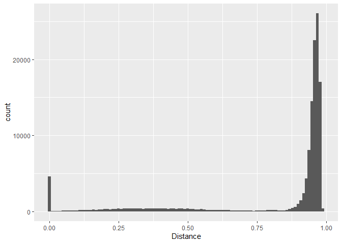
We may plot a histogram of these distances, to get a picture of how similar the proteins tend to be
fig3 <- ggplot(dst.tbl) +
  geom_histogram(aes(x = Distance), bins = 100)
print(fig3)
We notice:
- Some pairs are identical, and most of these are self-alignments. All
proteins are identical (
Distanceis 0.0) to themselves. - Many distance are large, close to 1.0. We could have lowered the
E-value threshold in
bDist()to eliminate many of these right away.
The distances below 0.75 are the ones we are interested in this time. In order to cluster we need to set some distance threshold somewhere, and from this histogram a value of 0.75 seems like a good start. This is a rather large threshold, and we should be prepared to use a smaller value if this results in very few and very large clusters.
If you have many genomes, say more than 100, you may find the reading of
the files takes quite some time. Then you may do this in a separate
step, using readBlastSelf() and readBlastPair() and save their
results to some .RData files. This means you can read chunks of files
and perhaps run it in parallel. These functions will return tables of
BLAST results that you bind together into one long table and use as
input to bDist() instead of the file names, using the argument
blast.tbl instead of blast.files in bDist(). Here is how we may do
it, using the small example:
self.tbl <- readBlastSelf(file.path("blast", list.files("blast", pattern = "txt$")))## readBlastSelf:
## ...received 55 blast-files...
## ...found 10 self-alignment files...
## ...returns 31259 alignment results
pair.tbl <- readBlastPair(file.path("blast", list.files("blast", pattern = "txt$")))## readBlastPairs:
## ...received 55 blast-files...
## ...found 45 alignment files who are NOT self-alignments...
## ...returns 115718 alignment results
dst.tbl <- bDist(blast.tbl = bind_rows(self.tbl, pair.tbl))## bDist:
## ...found 121923 alignments...
## ...where 4542 are self-alignments...
The self.tbl is never super-big, but the pair.tbl may have many
million rows. Instead of giving it all files to read, it may be possible
to speed things up by processing many chunks in parallell. Still, the
bDist() will need all rows in the end and you may run out of memory if
the number of gnomes is too large.
The bClust() uses classical hierarchical clustering based on the
distances we computed above. We can specify the linkage function to
use. The complete linkage is the ‘strictest’ way of clustering, in the
sense that no distance between two members can exceed the threshold we
specify. It is often a good choice to use
- A
completelinkage clustering - And a rather libral (large) threshold
The completelinkage means we have exact control of the ‘radius’ of our
clusters ore gene families. The other linkages are less transparent in
this sense.
Let us try this:
clst.blast <- bClust(dst.tbl, linkage = "complete", threshold = 0.75)## bClust:
## ...constructing graph with 4542 sequences (nodes) and 21504 distances (edges)
## ...found 627 single linkage clusters
## ...found 41 incomplete clusters
## 1 / 41 2 / 41 3 / 41 4 / 41 5 / 41 6 / 41 7 / 41 8 / 41 9 / 41 10 / 41 11 / 41 12 / 41 13 / 41 14 / 41 15 / 41 16 / 41 17 / 41 18 / 41 19 / 41 20 / 41 21 / 41 22 / 41 23 / 41 24 / 41 25 / 41 26 / 41 27 / 41 28 / 41 29 / 41 30 / 41 31 / 41 32 / 41 33 / 41 34 / 41 35 / 41 36 / 41 37 / 41 38 / 41 39 / 41 40 / 41 41 / 41
## ...ended with 678 clusters, largest cluster has 22 members
This results in 678 gene families or clusters. The largest cluster has 22 members, which is not very large given we have 10 genomes, and all core gene families should have at least 10 members. If many of the largest clusters become huge compared to the number of genomes, the threshold is probably too liberal (too large).
Note that the clustering vector clst.blast contains, in its names, the
unique information to identify a protein and the genome from which it
comes. Let us briefly have a look at which proteins belong to cluster 1:
print(clst.blast[clst.blast == 1])## GID1_seq1 GID10_seq1 GID2_seq1 GID3_seq1 GID4_seq1 GID5_seq1 GID6_seq1
## 1 1 1 1 1 1 1
## GID7_seq1 GID8_seq1 GID9_seq1
## 1 1 1
We notice this cluster has exactly one member from each genome (all 10
GID.tags), a ‘perfect’ core gene.
The fundamental data structure for many pan-genome analyses is the pan-matrix. This is simply a matrix with one row for each genome and one column for each gene cluster. The only input required is the clustering vector from above:
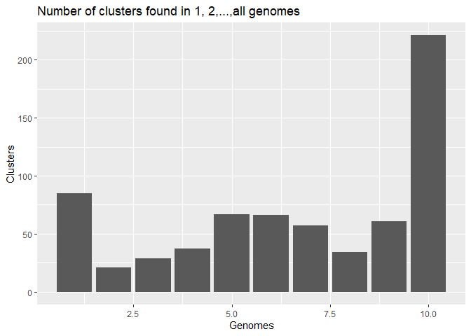
panmat.blast <- panMatrix(clst.blast)Once we have the pan-matrix, we can make a bar-chart over how many clusters are found in 1,2,…,all genomes:
tibble(Clusters = as.integer(table(factor(colSums(panmat.blast > 0),
                                          levels = 1:nrow(panmat.blast)))),
       Genomes = 1:nrow(panmat.blast)) %>%
  ggplot(aes(x = Genomes, y = Clusters)) +
geom_col() + labs(title = "Number of clusters found in 1, 2,...,all genomes")How big is the pan-genome? We are not talking about the number of gene clusters in the current sample, because this is just the number of columns in the pan-matrix. The size of the pan-genome is the number of gene clusters we would see if we collected all genomes of the species, not just the current sample. Will the number of clusters grow forever, or will it level out?
The heaps() function gives some estimate of pan-genome openness:
heaps.est <- heaps(panmat.blast, n.perm = 500)According to the theory the pan-genome is closed if the estimated
alpha is above 1.0:
print(heaps.est)## Intercept alpha
## 289.022258 1.704942
which is the case here. This means the growth of new gene clusters as we
sample more and more genomes tend to level off, see the Help-file for
heaps() for more details.
So how big does it look like this pan-genome will be? The chao() shed
some light on this:
print(chao(panmat.blast))## [1] 850
which is an estimate of the total number of gene clusters for this species. When based on only 10 genomes, this is a rather uncertain estimate!
An alternative estimate is found by fitting binomial mixture models to the data:
fitted <- binomixEstimate(panmat.blast, K.range = 3:8)## binomixEstimate: Fitting 3 component model...
## binomixEstimate: Fitting 4 component model...
## binomixEstimate: Fitting 5 component model...
## binomixEstimate: Fitting 6 component model...
## binomixEstimate: Fitting 7 component model...
## binomixEstimate: Fitting 8 component model...
By inspecting the fitted BIC.tbl we can see how many mixture
components is supported best by these data:
print(fitted$BIC.tbl)## # A tibble: 6 x 4
## K.range Core.size Pan.size BIC
## <dbl> <dbl> <dbl> <dbl>
## 1 3 217 756 2911.
## 2 4 101 864 2839.
## 3 5 6 897 2851.
## 4 6 28 890 2864.
## 5 7 0 1059 2876.
## 6 8 0 928 2890.
The minimum BIC-value is found at 4 components, indicating an optimum here. We also see that in this row the estimate of pan-genome size is 1160, and the size of the core-genome is 97.
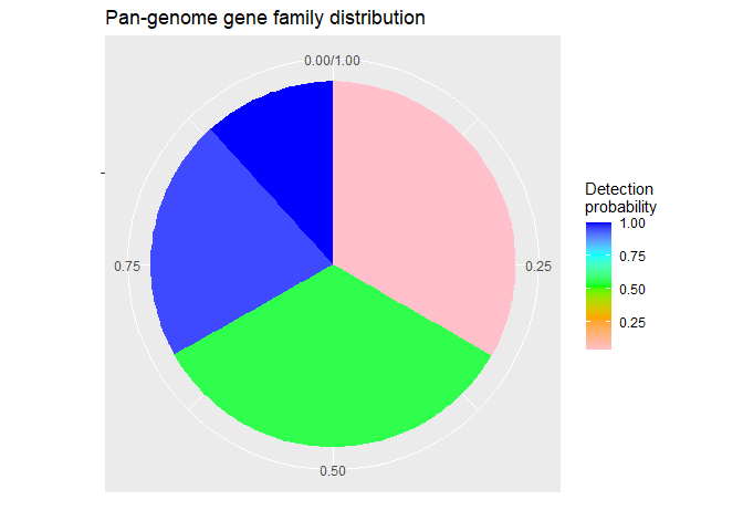
The 4 components means we can actually group gene clusters into 4 categories with respect to how frequent they tend to occur in the genomes. This may also be plotted:
ncomp <- 4
fig4 <- fitted$Mix.tbl %>%
  filter(Components == ncomp) %>%
  ggplot() +
  geom_col(aes(x = "", y = Mixing.proportion, fill = Detection.prob)) +
  coord_polar(theta = "y") +
  labs(x = "", y = "", title = "Pan-genome gene family distribution",
       fill = "Detection\nprobability") +
  scale_fill_gradientn(colors = c("pink", "orange", "green", "cyan", "blue"))
print(fig4)
We see that roughly half the pan-genome consists of the pink
‘cloud-genes’ with very low detection probability, i.e. gene clusters
seen in very few genomes only. Also, in addition to the core-genes
always observed, there is a component of almost-core-genes, seen in
almost all genomes. Note that in binomixEstimate() you may set the
core.detection.prob (slightly) lower than 1.0 to allow core-genes to
be absent from some genomes. This is reasonable if we have incomplete
genomes, genes may be there but is not detected due to incomplete
sequence data.
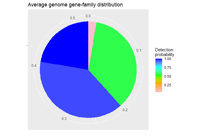
The figure above is for the entire pan-genome, but how does it look like in one (average) genome? Like this:
fig5 <- fitted$Mix.tbl %>%
  filter(Components == ncomp) %>%
  mutate(Single = Mixing.proportion * Detection.prob) %>%
  ggplot() +
  geom_col(aes(x = "", y = Single, fill = Detection.prob)) +
  coord_polar(theta = "y") +
  labs(x = "", y = "", title = "Average genome gene-family distribution",
       fill = "Detection\nprobability") +
  scale_fill_gradientn(colors = c("pink", "orange", "green", "cyan", "blue"))
print(fig5)
As expected, in a single genome the ‘cloud-genes’ (pink) are rare.
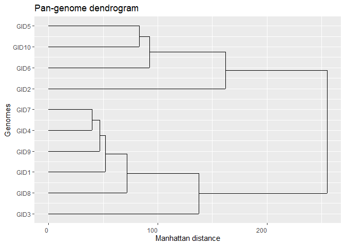
From the pan-matrix we may also compute distances between genomes:
d.man <- distManhattan(panmat.blast)and from these we make a dendrogram tree to visualize their relations:
library(ggdendro)
ggdendrogram(dendro_data(hclust(d.man, method = "average")),
             rotate = TRUE, theme_dendro = FALSE) +
  labs(x = "Genomes", y = "Manhattan distance", title = "Pan-genome dendrogram")
The Manhattan distance is simply how many gene clusters have differing
presence/absence status between two genomes, but remember the distances
displayed in the tree are average linkage distances between clusters.
Change the linkage by changing method = "average" in the call to
hclust().
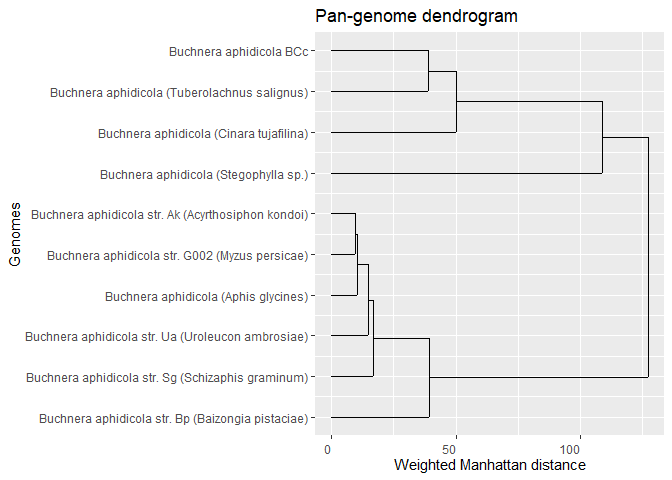
Since the ‘cloud-genes’ tend to be of a less reliable nature (gene
prediction errors), it may be a good idea to weight the distance such
that differences in the ‘shell-genes’ (green sectors above)
presence/absence becomes more important. Here is how we can do this, and
at the same time we also replace the GID.tag labels by their
corresponding Name:
pm <- panmat.blast                                                   # make a copy
rownames(pm) <- gnm.tbl$Name[match(rownames(pm), gnm.tbl$genome_id)] # new rownames
weights <- geneWeights(pm, type = "shell")
distManhattan(pm, weights = weights) %>%
  hclust(method = "average") %>%
  dendro_data() %>%
  ggdendrogram(rotate = TRUE, theme_dendro = FALSE) +
  labs(x = "Genomes", y = "Weighted Manhattan distance", title = "Pan-genome dendrogram")
There are of course many variations of this dendrogram, by using other distances, different weighting etc.
An alternative to the BLAST procedure above is to search all proteins for domains and group them by which sequence of domains they contain. The advantage is that we do not need to decide any thresholds, and the approach is robust to gene prediction errors, since rubbish genes tend not to contain any domains. The problem compared to the BLAST approach is lower resolution, and that not all proteins are grouped.
The HMMER software is needed here. This is only built for UNIX-like systems, but there are some possibilities of running it under windows as well, see its documentation. We also need a domain database to scan against, and the natural choice is the Pfam-A database. Any database based on the HMMER software is useful.
We assume you have downloaded and unpacked the Pfam-A.hmm file, stored
this in some folder and run hmmpress on it. We use the hmmerScan()
function to do the search:
pfam.db <- "~/projects/publicdata/Pfam/Pfam-A.hmm"
dir.create("pfam")
hmmerScan(file.path("faa", str_c(gnm.tbl$GenBank_ID, "_", gnm.tbl$genome_id, ".faa")),
          dbase = pfam.db,
          out.folder = "pfam")
Note that the content of pfam.db in the code above needs to be edited
to match where you have this database on your system.
Just like BLASTing, this is a time consuming step, and results are
stored in the subfolder pfam/ for later. If you add more genome later,
you simply re-run this code, and the existing result files will not be
re-computed.
First we read all results from the step above, i.e. the Pfam-A domains
found in all proteins. We also use the hmmerCleanOverlap() to discard
overlapping domains. In some cases two or more domains match the same
region of the protein. In such cases we only keep the best matching
domain.
pfam.files <- list.files("pfam", pattern = "txt$")
hmmer.tbl <- NULL
for(i in 1:length(pfam.files)){
  readHmmer(file.path("pfam", pfam.files[i])) %>%
    hmmerCleanOverlap() %>%
    bind_rows(hmmer.tbl) -> hmmer.tbl
}
The full table has 7403 rows, which is the number of times a protein has a hit against a domain. Many proteins have several domain hits. The domain sequence of a protein is the ordered sequence of domains appearing in it.
We cluster the proteins based on their domain sequences. Only proteins having identical domain sequences are in the same cluster:
clst.pfam <- dClust(hmmer.tbl)The number of clusters is simply the number of unique values in
clst.pfam
length(unique(clst.pfam))## [1] 669
Replace the clst.blast by this clst.pfam, and all examples above may
be repeated.
In some cases we would like to study in more detail the actual genes who
are present in 1,2,…, etc genomes, e.g. the core genes who are present
in all genomes. The function extractPanGenes() extracts genes found in
a specified number of genomes. Let us extract the genes found in 9 or 10
genomes based on the BLAST clustering from above:
core.tbl <- extractPanGenes(clst.blast, N.genomes = 9:10)This produces a table with 3 columns, listing these genes.
We can write the gene families to separate fasta files using the
geneFamilies2fasta() function. Let us put these into a new folder
named `core_fam’:
dir.create("core_fam")
geneFamilies2fasta(core.tbl, fasta.folder = "faa", out.folder = "core_fam")
This will create a fasta file for each gene family, and the file names contain the gene family (=cluster) and how many genomes it occurred in.
It is super simple to add the sequences yourself to a table like
core.tbl. The seq_tag column has the text that uniquely defines each
sequences in this study. By the following few code lines we read all
proteins, and add only those listed in the table:
lapply(list.files("faa", full.names = T), readFasta) %>%
  bind_rows() %>%
  mutate(seq_tag = word(Header, 1, 1)) %>%
  right_join(core.tbl, by = "seq_tag") -> core.seq.tbl
Notice how we use lapply() and readFasta() to read all fasta files
in one go, and then bind_rows() to make this into one big table. This
is possible since readFasta() returns fasta file content as a table.
Then we create a seq_tag column by using the first token in the
fasta Header, which is always the sequence tag if your files have been
prepared by panPrep().
Since the resulting table (core.tbl) has a Headerand Sequence
column, you may write it to a fasta file directly, using writeFasta().
If you use core.seq.tbl as argument to geneFamilies2fasta the
fasta.folder argument is ignored, and the already existing sequences
are used instead.
