TTitcombe / Basketball_Homography

Creating a Basketball Simulation Minimap from Single View Broadcast Data Using Applied Homography

Full Article Published: https://medium.com/mlearning-ai/developing-a-basketball-minimap-for-player-tracking-using-broadcast-data-and-applied-homography-433183b9b995

Initial Process

1. The inital input video is placed in the videos folder.
2. We then install our dependencies. This includes detectron2 and opencv. These dependencies allow us to track objects in a frame, determine what the object is and apply homography to the frames to convert the vectors from a 3D scale to a 2D one.
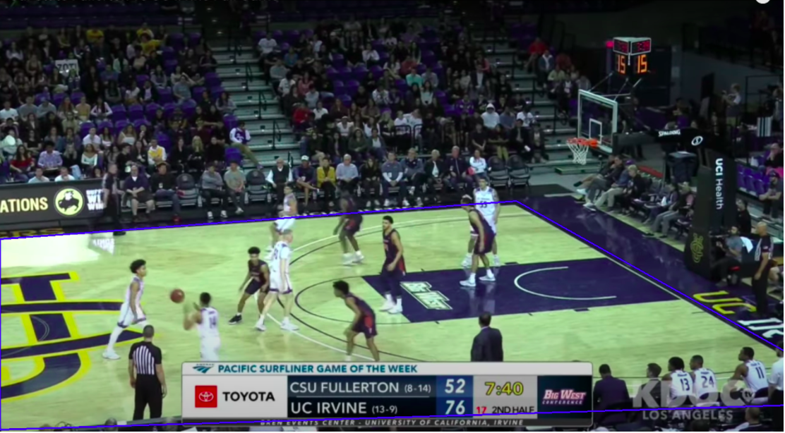
3. We then determine the dimensions of the court and display it as shown below. This is important as we will track the players by determining if their two-dimensional coordinates are within the court dimensions we have specified.
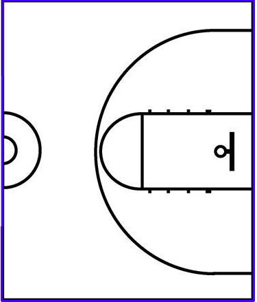
4. Now we need to take a 2D image of the court so we can translate the image frame onto the court. We have to specify the dimensions so we can proportionally transform the player coordinates accordingly. The court image is shown below.
5. Now we can apply homography function to reshape the frame to the same dimensions of the court image. The converted image is shown below.

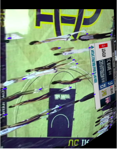
Notice the blue points next to each player. In order to do this we need to take the prediction boxes generated from detectron2 to generate coordinate points and images for each player. This is used to not only find the players on the court but to also determine the color value for player classification.

Player Classification and Final Process

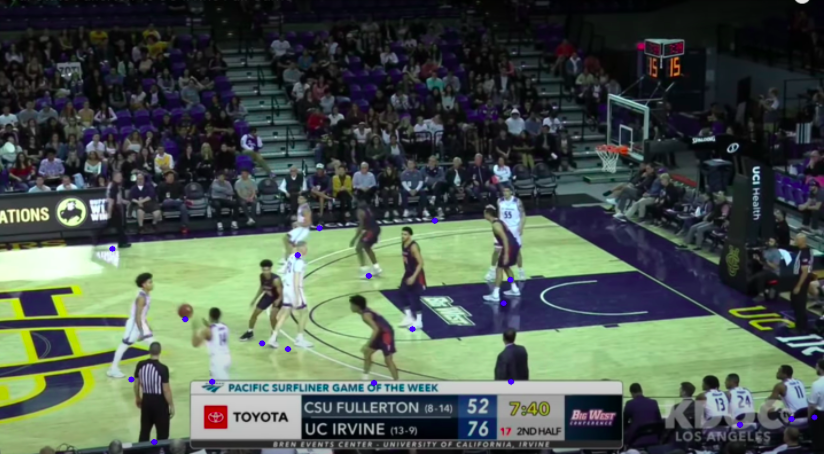
1. The prediction boxes are used in our drawPlayers method to find the center coordinates of the player on the court and draw these points as shown below.
2. Our create_images function is then used to create images of each player who was determined to be on the court and pass it into the images folder. For each frame that is passed into our final function, the images folder will be repopulated with the players who were on the court in that frame. Here is an example of one player we captured.

3. After the images folder is populated we grab each image and take a set of pixel values from the center of the image. We find the RGB values for each pixel coordinate and threshold the values to classify it as either the home team color or away team color. We take 5 pixel values, thus if the classified pixel colors are: blue, red, red, red, blue, the image will be classified as red. The get_info() and create_rbg_csv() accomplishes this task.
4. From there our final function drawPlayersOnCourt takes the data from the previous functions including transformed player coordinates to draw circles representing players onto the basektball court. Each frame is passed through these functions and written to an MP4 file using opencv.
5. A find_closest_player function maps the original points to the closest neighbor and draws a line to them to show the distance traveled.

Demo Output

view ouput_vid.mp4

Plans in the Future

1. Complete the team color classification and reduce noise in player movement.
2. Improve memory allocation optimization to handle larger videos.
3. Improve court dimensionality to reduce noise from the crowd.