
The objective of this project is to implement an end to end learning system which learns from manually driven scenarios how to drive safely around a circuit in a simulator. The CNN inputs are raw images and the output is the predicted steering angle.
The challenge of this project is not only developing a CNN model which is capable to drive the car around the trained track, but also to generalize the model in such a way that the car drives safely through scenarios it hasn't seen before (e.g. the mountain or the jungle track).
The following list gives a short overview about all relevant files and its purpose.
- model.py containing the script to create and train the model
- drive.py for driving the car in autonomous mode
- model.h5 containing a trained convolution neural network
- toolbox.py containing basic scripts to prepare the datasets (e.g. merging CSV files, reduced 0° steering angles, plot steering angle histograms, plot odometry signals over time, etc.)
- DataAugmentation.py containing functions to augment the dataset (e.g. image flipping, translation, brightness, shadows, etc.)
- BaseNetwork.py for basic network function like initialization, training and model storage
- LeNet.py containing the standard LeNet-5 model
- NvidiaFull.py containing a fully implemented NVIDIA model
- NvidiaLight.py containing a lightweight NVIDIA model (reduced number of convolutional and fully connected layers)
- VGG.py containing a basic VGG-16 model
- writeup.md summarizing the results
- video_track_1.mp4 autonomous driving behavior on track 1
- video_track_2.mp4 autonomous driving behavior on track 2 (jungle track)
I started to investigate a simple LeNet-5 model to get a first baseline. Additionally, I investigated the full NVIDIA CNN model because it's a well proven architecture for exactly this type of problem. In order to reduce the number of trainable weights and thus the training duration, I did some experiments with a "lightweight" NVIDIA model which has less convolutional and fully connected layers, and a reduced depth in each layer.
| Network | Link |
|---|---|
| LeNet-5 | http://yann.lecun.com/exdb/lenet/ |
| NVIDIA CNN | https://arxiv.org/pdf/1604.07316v1.pdf |
| NVIDIA "lightweight" CNN | Modified NVIDIA model (reduced number of convolutional and densed layers) |
The model uses an adam optimizer with max learning rate of 0.0001. The default learning rate of 0.001 was to big so that the mean squared error loss of the training and validation dataset stagnated already after the first epoch. For the batch size I chose 256 samples which could be easily loaded into memory on the AWS instance.
To find the best activation function, I tested all applied models with different activations like RELU, ELU, tanh. The ELU activation tend to extremely nervous steering angle predictions so that the car starts to bounce between the left and right lane boundary. The tanh activation often underestimated the steering angle. Best prediction results have been achieved with the RELU activation.
In addition, I tested different image input sizes and color spaces. I cropped the image to the ROI=[20, 60, 300, 138] in order to remove the hood and the landscape (e.g. trees, sky, etc.) which do not provide any beneficial input to the model. The crop on the left/right side has been introduced to reduce the influence of the replicated image areas induced by the image augmentation (see chapter Dataset Augmentation below for further details). Finally, I resized the image to 64x64 pixels to speed up the training process. Several test runs with different image sizes showed that the size have almost no influence on the prediction performance (at least in tested range and samples).

In order to generalize the model and to drive smoothly in the center of the lane on track 1 and in the center of the right lane on track 2, I heavily augmented the dataset by usage of left and right camera images, random translations, random shadow augmentations, random brightness changes, etc. All applied augmentations methods are explained in detail in chapter Creation of the Training Set & Training Process.
Every time I identified a section the car left the lane (e.g. sharp turns, bridge area, shadow sections, slopes, ...) I either tried to optimize the augmentation algorithms or collected additional recordings of these sections by the following rules.
- 4 times center line driving through critical section in forward direction
- 4 times center line driving through critical section in backward direction to balance the dataset
- 3-5 times recovery scenarios
All networks have been trained on an Amazon Web Services (AWS) EC2 g2.2xlarge instance with the following hardware configuration. The training time for the final NVIDA model took for one epoch with 30.000 samples in average 110 sec (1.8 min). The total training time took around 43 minutes.
- 8 vCPUs (Intel Xeon E5-2670)
- 1 GPU (NVIDIA 1536 CUDA processor with 4 GB video RAM)
- 15 GB RAM
- 60 GB SSD
After each epoch I stored the trained model because the validation loss is not a good indicator about how well the model drives in the simulator. It happened that a worse validation loss drives more stable and smoother than a lower one. Furthermore, the training has been stopped as soon as the validation loss hasn't been change for 3 consecutive epochs (for details see train() method in BaseNetwork.py).
checkpoint = ModelCheckpoint(filepath, monitor='val_loss', verbose=1, save_best_only=False, mode='min')
early_stopping = EarlyStopping(monitor='val_loss', patience=3, verbose=True)
The following table summarizes the results of the trained networks in the driving simulator. All networks have been trained with the same dataset. The number of epochs indicates the selected model checkpoint which performs best on track 1 and 2. To handle track 1 only, even a less number of epochs is completely sufficient (e.g. LeNet-5 needs 7 epochs to perform well on track 1).
The LeNet-5 model worked well in easy scenarios as they can be found on track 1 but cannot handle more challenging situations like hilly or shadow sections. The NVIDIA lightweight model performs better on track 2 compared to the simple LeNet-5 model but wasn't able to keep the car into the ego lane in sharp curves (steering angles >= 20°). The full NVIDIA model is able to handle all sections.
| Network | Epochs | Track 1 | Track 2 |
|---|---|---|---|
| LeNet-5 | 20 | good performance | Leaves the ego lane in hilly and shadow sections. |
| NVIDIA lightweight | 15 | good performance | Leaves the ego lane in sharp curves. Trouble with shadow sections. |
| NVIDIA Full | 24 | good performance | good performance |
The final model architecture (NvidiaFull.py) consists of a convolution neural network with the following layers and layer sizes. The RGB input images are cropped and resized to 64x64 pixels outside the model.
The first layer normalizes the image to a range between -0.5 and +0.5 by use of a Keras lambda layer. To introduce nonlinearity I chose for all convolutional and fully connected layers a RELU activation. To avoid overfitting the model contains 3 dropout layers with a drop rate of 50% in the fully connected layers.
| Layer | Depths/Neurons | Kernel | Activation | Pool Size | Stride | Border Mode | Output Shape | Params |
|---|---|---|---|---|---|---|---|---|
| Lambda | 3@64x64 | |||||||
| Convolution | 3 | 5x5 | RELU | 3@64x64 | 228 | |||
| Max pooling | 2x2 | 2x2 | same | 3@32x32 | ||||
| Convolution | 24 | 5x5 | RELU | 24@32x32 | 1824 | |||
| Max pooling | 2x2 | 2x2 | same | 24@16x16 | ||||
| Convolution | 36 | 5x5 | RELU | 36@16x16 | 21636 | |||
| Max pooling | 2x2 | 2x2 | same | 36@8x8 | ||||
| Convolution | 48 | 3x3 | RELU | 48@8x8 | 15600 | |||
| Max pooling | 2x2 | 1x1 | same | 48@4x4 | ||||
| Convolution | 64 | 3x3 | RELU | 64@4x4 | 27712 | |||
| Max pooling | 2x2 | 1x1 | same | 64@2x2 | ||||
| Flatten | 256 | |||||||
| Fully connected | 1164 | RELU | 1164 | 299148 | ||||
| Dropout 50% | 1164 | |||||||
| Fully connected | 100 | RELU | 100 | 116500 | ||||
| Dropout 50% | 100 | |||||||
| Fully connected | 50 | RELU | 50 | 5050 | ||||
| Dropout 50% | 50 | |||||||
| Fully connected | 10 | RELU | 10 | 510 | ||||
| Fully connected | 1 | 1 | 11 |
Total params: 488,219 Trainable params: 488,219 Non-trainable params: 0
Udacity provides a basic dataset with 8.036 samples recorded on track 1. It consist of a CSV file (see listing below) containing the path to center, left and right image, the steering angle, the throttle position, the brake force and the speed. The image size is 320x160 pixels (width x height). The steering angle is normalized to -1.0 and +1.0 which corresponds to an angle range of -25° to +25°.
center,left,right,steering,throttle,brake,speed
IMG_track_1_udacity/center_2016_12_01_13_30_48_287.jpg,IMG_track_1_udacity/left_2016_12_01_13_30_48_287.jpg,IMG_track_1_udacity/right_2016_12_01_13_30_48_287.jpg,0,0,0,22.14829
IMG_track_1_udacity/center_2016_12_01_13_30_48_404.jpg,IMG_track_1_udacity/left_2016_12_01_13_30_48_404.jpg,IMG_track_1_udacity/right_2016_12_01_13_30_48_404.jpg,0,0,0,21.87963
IMG_track_1_udacity/center_2016_12_01_13_31_12_937.jpg,IMG_track_1_udacity/left_2016_12_01_13_31_12_937.jpg,IMG_track_1_udacity/right_2016_12_01_13_31_12_937.jpg,0,0,0,1.453011
Exemplary left, center and right images in the Udacity dataset

Distribution of the steering angles in the Udacity dataset
The majority of samples (around 4.000 samples) are recorded with a steering angle close to 0°. With a median µ=0.1° the steering angles are well balanced. Looking on the the 3-sigma value, 99,73% of all steering angles are in the range of ±9.66° which is for track 1 sufficient but does not match the required range of track 2.
| Parameter | Value |
|---|---|
| Number of samples | 8.036 |
| Steering angle range | -23.57° .. +25.00° |
| ± 1-sigma (68.27%) | ± 3.23° |
| ± 2-sigma (95.45%) | ± 6.45° |
| ± 3-sigma (99.73%) | ± 9.66° |
| Median µ | 0.1017° |

To capture good driving behavior, I first recorded one lap forward and one lap backward on track 1 using center lane driving. Additionally, I recorded special scenes (e.g. curves with no markings, the bridge area, poles, etc.) which are underrepresented in the forwards/backwards recordings. The same procedure has been applied to track 2.
Distribution of the steering angles in the Udacity dataset
The table and histogram below show the combined dataset characteristics with Udacity's and own samples. The majority of samples (around 6.500 samples) are recorded with a steering angle close to 0° which is still far to much and will definitely lead to an bias during training. With a median µ=0.29° the steering angles are almost well balanced with a slight tendency to the right. Looking on the the 3-sigma value, 99,73% of all steering angles are in the range of ±26.6° which covers the whole steering angle range of ±25°. This is far better compared to the Udacity dataset.
| Parameter | Value |
|---|---|
| Number of samples | 42.989 |
| Steering angle range | -25.00° .. +25.00° |
| ± 1-sigma (68.27%) | ± 8.87° |
| ± 2-sigma (95.45%) | ± 17.74° |
| ± 3-sigma (99.73%) | ± 26.60° |
| Median µ | 0.2888° |

In order to recover from situations when the car accidentally drives too close to the road boundary or even off the track, I recorded a couple of recovery scenes. For that purpose, I placed the car on or very close to the left and right road boundary and smoothly steered back to the center of the lane. By this method the model learns how to recovery from unusual driving situations. The images below give an impression how a recovery scene looks like.


To increase the variety in the dataset in terms of road geometry (curve radius and slope), cast shadows, brightness and vehicle positions, I applied a couple of image augmentation methods. The images are randomly augmented in the generator() method in the BaseNetwork.py file.
The images below summarize the augmentation methods which basically change the color of the image. From left to right the original, the equalized histogram, the randomly applied brightness, the blur effect and the cast shadow effects are depicted.

In contrast to the color augmentation methods the images below show the results of the image flip, the image translation, the image rotation and the image perspective transformation methods. These methods not only augment the image itself but also the road geometry and the vehicle position. Hence the steering angle has to be adjusted accordingly (green line = original steering angle, red line = augmented steering angle).

My first idea to handle low contrast situations, like dark sections and cast shadows especially on track 2, was to apply an adaptive histogram equalization (CLAHE) to the RGB image as implemented in equalize_histogram(image). Because my model uses full RGB images, I applied the method on each RGB channel separately.
The brightness augmentation method random_brightness(image, probability=1.0) randomly changes the brightness of an image with the given probability. To change the brightness of a RGB image I converted it to the HSV color space and randomly adjusted the V channel. HSV stands for hue, saturation and value. HSV is also known as HSB (B for brightness).
Some other Udacity students made good experiences with blurred images which shall reduce the influence of cast shadows. Some cast shadows produces sharp edges in an image which might lead to errors in the predicted steering angle. The blur effect softens these sharp edges. One negative effect is that it blurs every structure which in the end might be important for the network to understand the current scenario. I implemented a basic blurring algo based on a 3x3 normalized box filter in the random_blur(image, probability=1.0) method.
The method random_shadow(image, probability=1.0) applies random cast shadows with a random intensity and the given probability. The method supports two different types of shadows. The two left images shows the first type whereas the four images on the right side depict the second type of shadow.

The easiest way to triple the number of samples in the dataset is to use the left and right camera images. Due to the lateral offset of the camera mounting position from the vehicle's center axis you get two additional offsets from the actual driving path. I corrected the steering angle by +6.25° for the left image and -6.25° for the right image.
The method flip_image_horizontally(image, steering_angle, probability=1.0, lr_bias=0.0) randomly flips the image horizontally and inverts the steering angle accordingly by the given probability. Furthermore, the lr_bias parameter allows to shift the flip tendency more to the left or more to the right. This allows to manually balance the steering angle distribution in the dataset.

(green line = original steering angle, red line = inverted steering angle)
The method random_translation(image, steering_angle, max_trans, probability=1.0) randomly translates the image in all four directions (upwards, downwards, left and right) with the given probability. The max_trans parameter defines the max applied translation in x- and y-direction.
The translation to left and right corresponds to different vehicle position within the lane whereas the translation in up-/downwards direction imitates different slopes of the roadway. The steering angle is only changed for translations into x-direction by 0.07°/pixel.

(green line = original steering angle, red line = augmented steering angle)
The method random_rotation(image, steering_angle, max_rotation, probability=1.0) randomly rotates the image around the center, bottom point of the image by the given probability. The max_rotation parameter limits the applied rotation angle.
The rotation of the image corresponds to the bank angle of the roadway. The steering angle is corrected by 0.3° per 1° image rotation.

(green line = original steering angle, red line = augmented steering angle)
The method random_perspective_transformation(image, steering_angle, max_trans, probability=1.0) randomly applies a perspective transformation with the given probability. The max_trans parameter limits the applied transformation in x- and y-direction.
A perspective transformation in x-direction changes the curve radius and in y-direction changes the roadway slope. The steering angle is only adjusted for perspective transformations in x-direction by 0.11°/pixel.

(green line = original steering angle, red line = augmented steering angle)
Not all implemented augmentation methods improved my model behavior as expected. Some even introduced unstable steering angle predictions like the histogram equalization. After a long empirical phase I decided to apply the following augmentation methods. The generator() method combines all methods randomly while training the model. Thereby the generator is able to create an unlimited number of unique training and validation samples.
- Usage of center, left and right images
- Random translations (dx_max=70 pixel, dy_max=30 pixel, probability=0.5)
- Random cast shadows (probability=0.5)
- Random brightness (probability=0.5)
- Random flip (probability=0.5, lr_bias=0.0)
- All possible combinations of these methods
In addition to that, I chose a distribution of 60% augmented images and 40% original images. To reduce the bias towards 0° steering angles I reduced the number of samples in the range of ±0.1° by 90%. The normed histogram shows the steering angle distribution of the reduced dataset and the online generated ones.


The final dataset consists of 37.348 well balanced samples which I split up into a training (80%) and a validation (20%) dataset. The steering angle range is bigger than the angle range the simulator accepts. These angles will be limited to ±25° in a later step.
| Parameter | Value |
|---|---|
| Number of samples | 37.348 |
| Steering angle range | -36.14° .. +35.72° |
| ± 1-sigma (68.27%) | ± 10.41° |
| ± 2-sigma (95.45%) | ± 20.83° |
| ± 3-sigma (99.73%) | ± 31.24° |
| Median µ | 0.1515° |
The NVIDA model trained with the dataset as described above showed the best performance on track 1 and 2.
You-Tube Links of track 1 and 2 results:
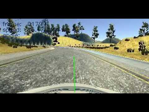
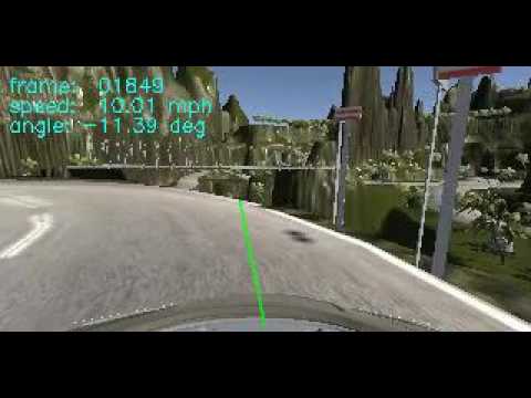
The diagram below depicts the trained and predicted steering angles of one round on track 1. The prediction is very close to the ground truth data but shows more jitter.

The project demonstrated that almost 90% is about composing a well balanced and well reasoned dataset. Only 10% of the total development effort was about CNN implementation.
The results clearly prove the potential of an end to end learning approach. Nevertheless, for real world applications it needs much more than just collecting data and train a network. To ensure the safety aspect under all possible conditions and unexpected events in real traffic situations (especially in urban areas) new methods to test and to validate such systems have to be introduced.