The purpose of this repository is to replicate the Jean et. al. (2016) paper (see papers/jean_et_al.pdf and papers/aaai16.pdf) using only Python3 and PyTorch. These more up-to-date tools and instructions should help anyone trying to recreate and build-off this work.
The purpose of the paper was to use abundant sources of data (namely satellite imagery and nightlights data) to predict poverty levels at a local level (on the order of a single village). For some background, every few years the World Bank conducts surveys in developing countries to understand their living situations. As you might expect, this process is very time-consuming. If we can make a model that only uses abundant sources of data to predict values that otherwise have to be measured through expensive human efforts, then several possibilities arise:
- prediction during "off-years" (when no surveys are collected)
- real-time monitoring of poverty conditions
- potential for early-warning systems
Note 1: all scripts are put in Jupyter Notebook (.ipynb) files to encourage exploration and modification of the work.
Note 2: I only work with data from Malawi
I recommend creating a virtual environment for this project. I prefer using Anaconda.
First run:
git clone https://github.com/jmather625/predicting-poverty-replication
conda create -n <ENV_NAME> python=3.7 pip gdal
conda activate <ENV_NAME>
conda install pytorch torchvision -c pytorch
pip install -r requirements.txt
The libraries that are most likely to fail are gdal and geoio. If a requirement fails to install, first make sure you follow this install procedure exactly. Using pip to install GDAL did not work for me, and the only way I got it to install was by including it when I first make the conda environment (hence pip gdal). Also, there are several Stack Overflow posts on these issues, so hopefully one will work on your machine.
If you want to run Jupyter Notebooks in an environment, run the following inside the environment:
pip install --user ipykernel
python -m ipykernel install --user --name=<ENV_NAME>
Then, set the kernel for all the Jupyter files to whatever your <ENV_NAME> is.
To allow tqdm (the progress bar library) to run in a Jupyter Notebook, also run:
conda install -c conda-forge ipywidgets
Additionally, you need to get the LSMS survey data from the world bank. Download the 2016-2017 Malawi survey data from https://microdata.worldbank.org/index.php/catalog. The World Bank wants to know how people use their data, so you will have to sign in and explain why you want their data. Query 'LSMS' and filter the years to help find the data. The title of the data when I downloaded it was Fourth Integrated Household Survey 2016-2017. If you look at the data description tab, you should see a huge list of files starting with HH_Metadata. Navigate to Get Microdata to download the data. Make sure to download the Stata version. Unzip the downloaded Malawi data into countries/malawi_2016/LSMS/.
Lastly, you need to get an api key from Google's Static Maps API service. Save it to api_key.txt in the root directory.
Run the Jupyter files in the following order:
scripts/download_nightlights_data.ipynb
scripts/process_survey_data.ipynb
scripts/download_images.ipynb
scripts/train_cnn.ipynb
scripts/predict_consumption.ipynb
In the code itself you should see some comments and lines explaining ever step. Couple points:
- the image download step will take the longest amount of time (about 7,000 images per hour)
- if you are working on a VM like Google's Deep Learning VM, connections can close after extended periods of time. This doesn't stop the script itself from running, but there's no way to see the progress bar in the notebook.
- training the CNN on CPU is something you should try to avoid. Training the CNN took under 30 minutes on a single GPU, and a forward pass to extract features took under 10 minutes. On CPU, those runtimes are at least an order of magnitude higher.
Besides training the CNN from scratch, you can also do one of the following:
I don't recommend doing this because you will need to setup Google's protocol buffers. This link may help:
https://github.com/protocolbuffers/protobuf/tree/master/python. First, download weights from https://www.dropbox.com/s/4cmfgay9gm2fyj6/predicting_poverty_trained.caffemodel?dl=0 into scripts/setup_existing_model/. Then, run the script in scripts/setup_existing_model/forward_pass.ipynb. Finally, run scripts/predict_consumption.ipynb.
Download the model I trained from https://drive.google.com/drive/folders/1gZZ1NoKaq43znWIBjzmrLuMQh4uzu9qn?usp=sharing and put it into the models directory. It should be named trained_model.pt. Then run scripts/predict_consumption.ipynb.
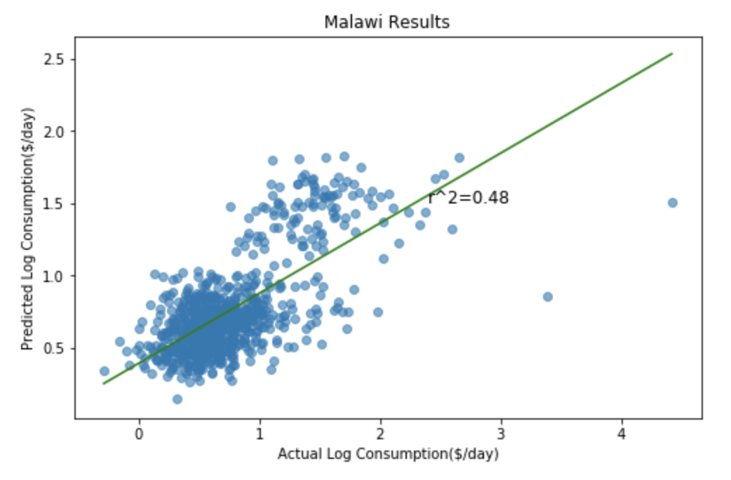
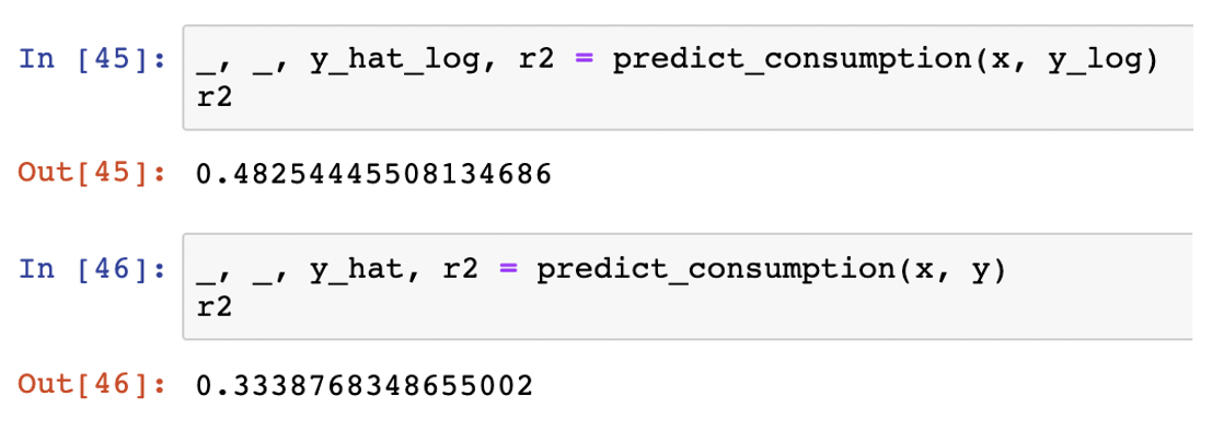
As a way to see how good the model is, I extract all features from the LSMS survey that an image could possibly recognize and use them to predict consumption. This serves as a "gold standard" for any image-based model. It turns out that the CNN model performs almost as well as this gold standard!
- Run
gold_standard/remote_features_survey_model.ipynb
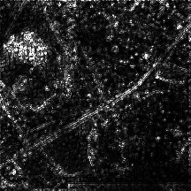
Activation maps are a good way to visually depict what a CNN focuses on.
- Run
activation_maps/visualize_cnn.ipynb
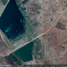
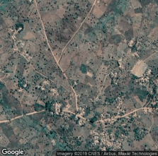
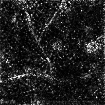
Big thanks to https://github.com/utkuozbulak/pytorch-cnn-visualizations for making CNN visualizations easier. I borrowed one technique, feel free to try more. Here are two examples:
Because the number of images far exceeds how many I can feasibly hand-check, it is difficult to make generalizations about what the model focuses on. That being said, roads tend to be a key area of focus, and bodies of water tend to be identified. Urban development/housing also seem to be important to the model, but activation maps outline them less clearly and distinctly than roads.
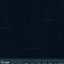
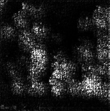
However, the model does not seem to be especially robust. The image below was downloaded via my script and appears to be during nighttime, therefore hold little visual information. Nevertheless, the activation maps are still bright with meaningless information.
This section is meant to explain at a high level the procedure that the paper follows.
- Download LSMS data. This data tells us a lot of low-level information about developing countries. This includes consumption, which is the variable we try to predict. Consumption is the dollars spent on food per day. $1.90 is the global poverty line.
- Download nightlights data. This data is hosted by the NOAA and can be downloaded for free. I use a geo-raster library to convert an input lat/long into pixel locations onto the array that is downloaded.
- Generate cluster aggregates for information. A cluster is defined as a 10km x 10km region enclosing a given central lat/long (which itself comes from the LSMS data). This means we aggregate values like consumption and nightlights across various lat/longs in a cluster.
- Transfer learn train VGG on the images to predict the nightlight bins.
- Compute the 4096 size feature vector (right before it is condensed into classification) for each image. Average these across a cluster.
- Assemble a dataset of clusters where you try to predict consumption (rather log consumption) from the aggregate feature vector per cluster. Use Ridge Regression.
You can reach me via email at jatinm2@illinois.edu
