SimonTreillou / TaylorDiag.jl

Github repo about Taylor diagram implementation in Julia.

TaylorDiag

What is a Taylor diagram

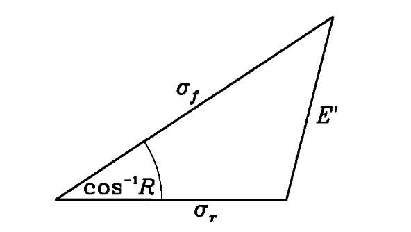
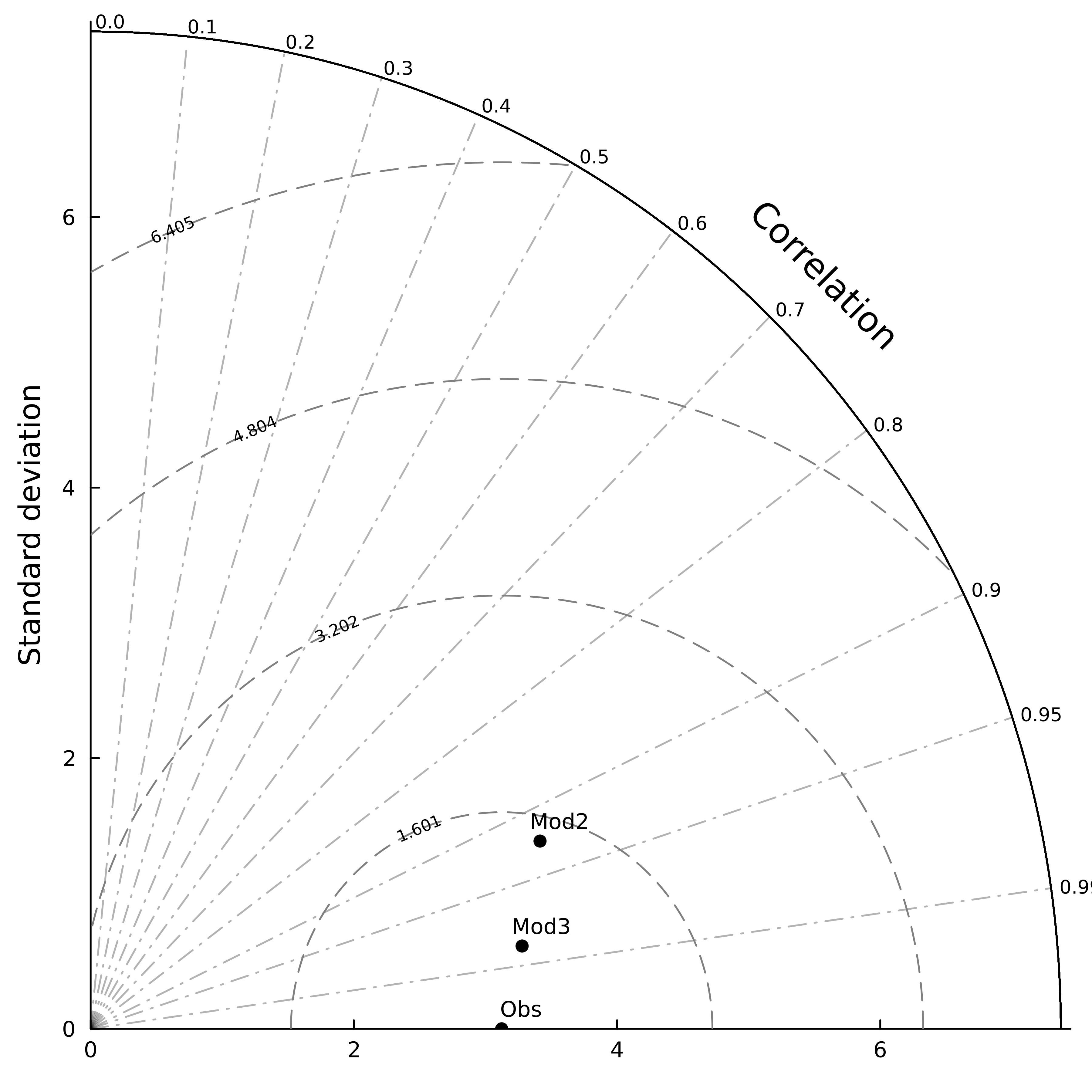
A Taylor diagram is a diagram designed by Karl E. Taylor [1], indicating the realism of models/representations. It is a really powerful tool because of the information displayed in a single diagram: the correlation coefficient (quantifying the pattern similarity between reference and model), the RMSE (quantifying the difference, without differentiating difference due to pattern and difference due to amplitude) and standard deviation (quantifying the amplitude and deviation). This diagram is well-known in earth sciences and climate sciences (e.g. oceanography, meteorology) but would benefit from being known in others scientific fields.

Given $f$ and $r$ two variables, $r$ being the reference, and $\sigma_f$ and $\sigma_r$ their respective standard deviations, the correlation coefficient R reads as :

$$ R = \frac{ \frac{1}{N} \sum_n (f_n - \bar{f}) (r_n - \bar{r})}{\sigma_f \sigma_r}$$

The RMS difference E reads as :

$$E = [ \frac{1}{N} \sum_n (f_n - r_n)^2 ]^{1/2}$$

and can be separated in two parts : $E^2 = \bar{E}^2 + E'^2$. $\bar{E} = \bar{f} - \bar{r}$ is the overall bias and the centered pattern RMS difference $E'$ is :

$$\sqrt{E'} = \frac{1}{N} \sum_n [(f_n - \bar{f}) - (r_n - \bar{r})]^2$$

Taylor (2001) then showed that these scores are related using the following equation :

$$E'^2 = \sigma^2_f + \sigma_r^2 - 2 \sigma_f \sigma_r R$$

$From \space Taylor \space (2001) - Figure \space 1$

How to use

You first need to add the package to your library.

using Pkg
Pkg.add("TaylorDiag")
using TaylorDiag

Example

using Random
using TaylorDiag

# We first build observations (e.g. reference) using random distribution
obs = 10*rand(10)

# Then we build "modeled" datasets (here the observations with random noise)
mod = obs + rand(10)*4
mod2 = obs + rand(10)*2

# We compute standard deviations (S), root mean squared deviations (R)
# and correlations (C)
S = [STD(obs),STD(mod), STD(mod2)]
R = [RMSD(obs,obs),RMSD(obs,mod), RMSD(obs,mod2)]
C = [COR(obs,obs),COR(obs,mod),COR(obs,mod2)]

# We then plot the Taylor diagram, here without special names added
taylordiagram(S,C)

# Here with automatic computation of the standard deviations 
# and correlation coefficients (plot not shown)
taylordiagram([obs,mod,mod2])

# Here with special names added (plot not shown)
names = ["Data1", "Data2", "Data3"]
taylordiagram(S,C,names)

# Here with special markers
markerz = [:star, :circle, :circle]
taylordiagram(S,C,markerz)

# Here with options and collections directly used as inputs (STD and C computations are automatic)
Cs = [obs,mod,mod2]
taylordiagram(Cs;figsize=600,dpi=600,pointcolor=:black,pointfontsize=8,correlationcolor=:red,freRMS=10,normalize=true)

Roadmap

• Statistics tests
• Write functions descriptions
• Add reference
• Write quick-quick documentation on the README
• Clean-up
• Add plotting options
• Normalized plot
• Reduced angle plot
• Use RecipesBase.jl
• Add examples
• Docs
• Improve 180° plot
• New skill scores from Taylor 2001
• Add RMSD on the plot
• List what next: see reference
• Add API
• Correlation lines size problem

Contributing

Contributions are welcome. Please make a pull request so the community can enjoy it!

See contributor's guide badge for more informations.

References

[1] Taylor, K. E. (2001). Summarizing Multiple Aspects of Model Performance in a Single Diagram Journal of Geophysical Research: Atmospheres 106, nᵒ D7 (2001): 7183‑92. https://doi.org/10.1029/2000JD900719.