Shinnnyshinshin / OlympicsAthletes

EDA Project for OlympicsAthletes

Initial Analysis of Olympic Data

Exploratory Analyis

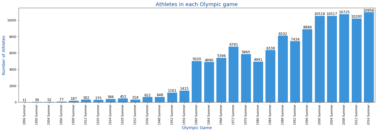
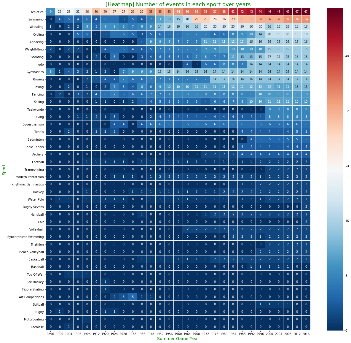
• how have the olympic games grown over the years?
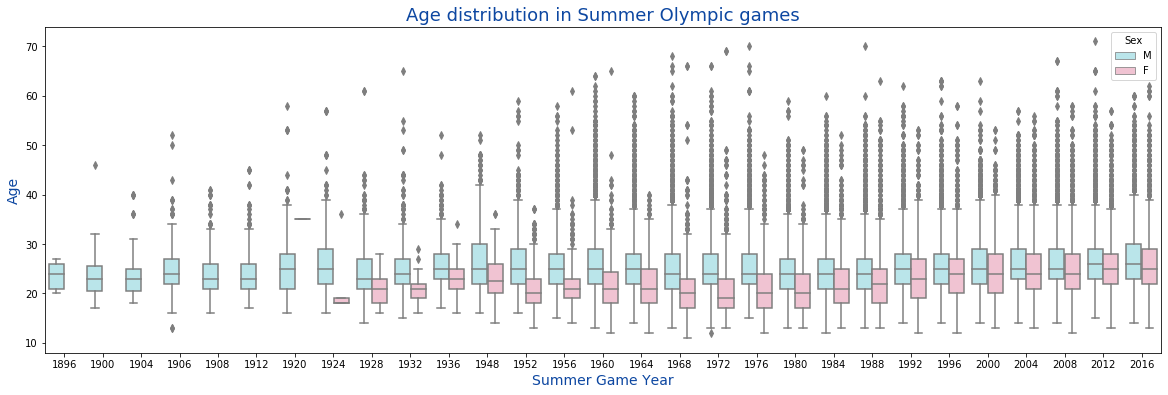
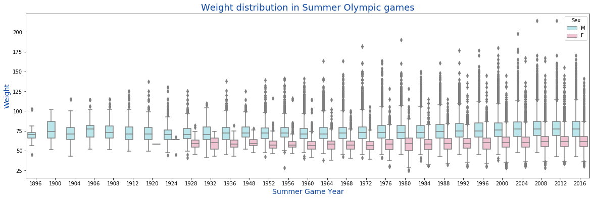
• how have athletes changed over the years

import numpy as np # linear algebra
import pandas as pd # data processing, CSV file I/O (e.g. pd.read_csv)

import seaborn as sns
import matplotlib.pyplot as plt
%matplotlib inline

import os

athlete = pd.read_csv('input/athlete_events.csv')
noc = pd.read_csv('input/noc_regions.csv')

print('Athlete data: \nRows: {}\nCols: {}'.format(athlete.shape[0],athlete.shape[1]))
print(athlete.columns)

print('\nNOC data: \nRows: {}\nCols: {}'.format(noc.shape[0],noc.shape[1]))
print(noc.columns)

Athlete data: 
Rows: 271116
Cols: 15
Index(['ID', 'Name', 'Sex', 'Age', 'Height', 'Weight', 'Team', 'NOC', 'Games',
       'Year', 'Season', 'City', 'Sport', 'Event', 'Medal'],
      dtype='object')

NOC data: 
Rows: 230
Cols: 3
Index(['NOC', 'region', 'notes'], dtype='object')

Let's look at the first entries of the NOC data and Athlete Data

athlete.head()

<style scoped> .dataframe tbody tr th:only-of-type { vertical-align: middle; }

.dataframe tbody tr th {
    vertical-align: top;
}

.dataframe thead th {
    text-align: right;
}

</style>

	ID	Name	Sex	Age	Height	Weight	Team	NOC	Games	Year	Season	City	Sport	Event	Medal
0	1	A Dijiang	M	24.0	180.0	80.0	China	CHN	1992 Summer	1992	Summer	Barcelona	Basketball	Basketball Men's Basketball	NaN
1	2	A Lamusi	M	23.0	170.0	60.0	China	CHN	2012 Summer	2012	Summer	London	Judo	Judo Men's Extra-Lightweight	NaN
2	3	Gunnar Nielsen Aaby	M	24.0	NaN	NaN	Denmark	DEN	1920 Summer	1920	Summer	Antwerpen	Football	Football Men's Football	NaN
3	4	Edgar Lindenau Aabye	M	34.0	NaN	NaN	Denmark/Sweden	DEN	1900 Summer	1900	Summer	Paris	Tug-Of-War	Tug-Of-War Men's Tug-Of-War	Gold
4	5	Christine Jacoba Aaftink	F	21.0	185.0	82.0	Netherlands	NED	1988 Winter	1988	Winter	Calgary	Speed Skating	Speed Skating Women's 500 metres	NaN

noc.head()

<style scoped> .dataframe tbody tr th:only-of-type { vertical-align: middle; }

.dataframe tbody tr th {
    vertical-align: top;
}

.dataframe thead th {
    text-align: right;
}

</style>

	NOC	region	notes
0	AFG	Afghanistan	NaN
1	AHO	Curacao	Netherlands Antilles
2	ALB	Albania	NaN
3	ALG	Algeria	NaN
4	AND	Andorra	NaN

Filter on athletes with incomplete data

Since we are trying eventually use the data from each individual athlete to predict the sport they are participating in, we are going to filter on incomplete data.

athlete_filt = athlete[(athlete['Sex'].notnull()) & (athlete['Age'].notnull()) & (athlete['Height'].notnull())  & (athlete['Weight'].notnull()) & (athlete['NOC'].notnull()) & (athlete['Year'].notnull()) & (athlete['Season'].notnull()) & (athlete['Sport'].notnull())]

#AthletesFiltered_Summer = athlete_filt.loc[(athlete_filt['Season'].isin(["Summer"])) & (athlete_filt['Year'] >= 1968)]
AthletesFiltered_Summer = athlete_filt.loc[(athlete_filt['Season'].isin(["Summer"]))]

print(AthletesFiltered_Summer.shape) 

athlete = AthletesFiltered_Summer

(166706, 15)

Initial Plotting (How have the games changed in the last 50 years?)

games_athletes = athlete.pivot_table(athlete, index=['Games'], aggfunc=lambda x: len(x.unique())).reset_index()[['Games','ID']]
fig, ax = plt.subplots(figsize=(22,6))
a = sns.barplot(x='Games', y='ID', data=games_athletes, ax=ax, color="#2196F3")
a.set_xticklabels(labels=games_athletes['Games'],rotation=90)

for p in ax.patches:
    ax.text(p.get_x() + p.get_width()/2., p.get_height(), '%d' % int(p.get_height()), 
            fontsize=12, color='black', ha='center', va='bottom')

ax.set_xlabel('Olympic Game', size=14, color="#0D47A1")
ax.set_ylabel('Number of Athletes', size=14, color="#0D47A1")
ax.set_title('Athletes in each Olympic game', size=18, color="#0D47A1")

plt.show()

sport_year = athlete[athlete['Season']=='Summer'].pivot_table(athlete, index=['Year','Sport'], aggfunc=lambda x: len(x.unique())).reset_index()[['Year','Sport','Event']]
sport_year = sport_year.pivot("Sport", "Year", "Event")
sport_year.fillna(0,inplace=True)
sport_year = sport_year.reindex(sport_year.sort_values(by=2016, ascending=False).index)
f, ax = plt.subplots(figsize=(20, 20))
sns.heatmap(sport_year, annot=True, linewidths=0.05, ax=ax, cmap="RdBu_r")
ax.set_xlabel('Summer Game Year', size=14, color="green")
ax.set_ylabel('Sport', size=14, color="green")
ax.set_title('[Heatmap] Number of events in each sport over years', size=18, color="green")
plt.show()

How have the athletes changed?

• We are initially going to look at 3 simple metrics, Age, Weight and Height

fig, ax = plt.subplots(figsize=(20,6))
a = sns.boxplot(x="Year", y="Age", hue="Sex", palette={"M": "#B2EBF2", "F":"#F8BBD0"}, data=athlete[athlete['Season']=='Summer'], ax=ax)
        
ax.set_xlabel('Summer Game Year', size=14, color="#0D47A1")
ax.set_ylabel('Age', size=14, color="#0D47A1")
ax.set_title('Age distribution in Summer Olympic games', size=18, color="#0D47A1")
plt.show()

fig, ax = plt.subplots(figsize=(20,6))
a = sns.boxplot(x="Year", y="Weight", hue="Sex", palette={"M": "#B2EBF2", "F":"#F8BBD0"}, data=athlete[athlete['Season']=='Summer'], ax=ax)
        
ax.set_xlabel('Summer Game Year', size=14, color="#0D47A1")
ax.set_ylabel('Weight', size=14, color="#0D47A1")
ax.set_title('Weight distribution in Summer Olympic games', size=18, color="#0D47A1")
plt.show()

fig, ax = plt.subplots(figsize=(20,6))
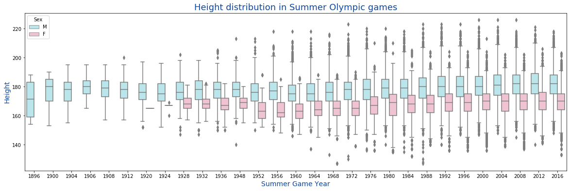
a = sns.boxplot(x="Year", y="Height", hue="Sex", palette={"M": "#B2EBF2", "F":"#F8BBD0"}, data=athlete[athlete['Season']=='Summer'], ax=ax)
        
ax.set_xlabel('Summer Game Year', size=14, color="#0D47A1")
ax.set_ylabel('Height', size=14, color="#0D47A1")
ax.set_title('Height distribution in Summer Olympic games', size=18, color="#0D47A1")
plt.show()

fig, ax = plt.subplots(figsize=(20,6))
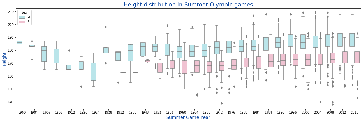
a = sns.boxplot(x="Year", y="Height", hue="Sex", palette={"M": "#B2EBF2", "F":"#F8BBD0"}, data=athlete[(athlete['Season']=='Summer') & (athlete['Sport']=="Swimming")], ax=ax)
        
ax.set_xlabel('Summer Game Year', size=14, color="#0D47A1")
ax.set_ylabel('Height', size=14, color="#0D47A1")
ax.set_title('Height distribution in Summer Olympic games', size=18, color="#0D47A1")
plt.show()

Now for a predictive model

# Let's if we can predict the sport of an athlete based on their body measurements

AthletesFiltered_Summer = athlete_filt.loc[(athlete_filt['Season'].isin(["Summer"])) & (athlete_filt['Year'] >= 1968)]
print(AthletesFiltered_Summer.shape) 

(142506, 15)

# number of athletes per sport

athletes_ps = AthletesFiltered_Summer[["Sport"]]
athletes_ps = athletes_ps["Sport"].value_counts()


#https://pandas.pydata.org/pandas-docs/stable/reference/api/pandas.Series.to_frame.html
athletes_per_sport = pd.DataFrame({"Sport":athletes_ps.index, "Athletes":athletes_ps.values})

fig, ax = plt.subplots(figsize=(30,6))
a = sns.barplot(x='Sport', y='Athletes', data=athletes_per_sport, ax=ax, color="#2196F3")
a.set_xticklabels(labels=athletes_per_sport['Sport'],rotation=90)

for p in ax.patches:
    ax.text(p.get_x() + p.get_width()/2., p.get_height(), '%d' % int(p.get_height()), 
            fontsize=12, color='black', ha='center', va='bottom')

ax.set_xlabel('Sport', size=14, color="#0D47A1")
ax.set_ylabel('Number of Athletes', size=14, color="#0D47A1")
ax.set_title('Athletes per Sport', size=18, color="#0D47A1")
plt.show()

Look a little more into the Athletics sport

As we see in the graph that the sport is athletics, which is a combination of many sports that are part of the track and field.

https://tokyo2020.org/en/games/sport/olympic/athletics/

Event Programme

• 100m (Men/Women)
• 200m (Men/Women)
• 400m (Men/Women)
• 800m (Men/Women)
• 1,500m (Men/Women)
• 5,000m (Men/Women)
• 10,000m (Men/Women)
• 110m Hurdles (Men)
• 100m Hurdles (Women)
• 400m Hurdles (Men/Women)
• 3,000m Steeplechase (Men/Women)
• 4 x 100m Relay (Men/Women)
• 4 x 400m Relay (Men/Women)
• 4 x 400m Mixed Relay

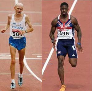
One concern that I have is that sprinters (100m and 200m) have very different body-types than mid and long-distance runners (10,000m) and this might make the categorization difficult.

# now let's do the actual filtering. 
ToFilter = ['Swimming', 'Gynmastics']

AthletesFiltered_Summer_Sports = AthletesFiltered_Summer.loc[AthletesFiltered_Summer['Sport'].isin(ToFilter)]

AthletesFiltered_Summer_Sports.head()

<style scoped> .dataframe tbody tr th:only-of-type { vertical-align: middle; }

.dataframe tbody tr th {
    vertical-align: top;
}

.dataframe thead th {
    text-align: right;
}

</style>

	ID	Name	Sex	Age	Height	Weight	Team	NOC	Games	Year	Season	City	Sport	Event	Medal
100	36	Stefan Remco Aartsen	M	21.0	194.0	78.0	Netherlands	NED	1996 Summer	1996	Summer	Atlanta	Swimming	Swimming Men's 100 metres Butterfly	NaN
101	36	Stefan Remco Aartsen	M	21.0	194.0	78.0	Netherlands	NED	1996 Summer	1996	Summer	Atlanta	Swimming	Swimming Men's 200 metres Butterfly	NaN
102	36	Stefan Remco Aartsen	M	21.0	194.0	78.0	Netherlands	NED	1996 Summer	1996	Summer	Atlanta	Swimming	Swimming Men's 4 x 100 metres Medley Relay	NaN
103	36	Stefan Remco Aartsen	M	25.0	194.0	78.0	Netherlands	NED	2000 Summer	2000	Summer	Sydney	Swimming	Swimming Men's 100 metres Butterfly	NaN
104	36	Stefan Remco Aartsen	M	25.0	194.0	78.0	Netherlands	NED	2000 Summer	2000	Summer	Sydney	Swimming	Swimming Men's 200 metres Butterfly	NaN

So here is what we did instead

# now let's do the actual filtering. 
ToFilter = ['Cycling', 'Rowing']

AthletesFiltered_Summer_Sports = AthletesFiltered_Summer.loc[AthletesFiltered_Summer['Sport'].isin(ToFilter)]

AthletesFiltered_Summer_Sports.head()

<style scoped> .dataframe tbody tr th:only-of-type { vertical-align: middle; }

.dataframe tbody tr th {
    vertical-align: top;
}

.dataframe thead th {
    text-align: right;
}

</style>

	ID	Name	Sex	Age	Height	Weight	Team	NOC	Games	Year	Season	City	Sport	Event	Medal
92	30	Pepijn Aardewijn	M	26.0	189.0	72.0	Netherlands	NED	1996 Summer	1996	Summer	Atlanta	Rowing	Rowing Men's Lightweight Double Sculls	Silver
93	30	Pepijn Aardewijn	M	30.0	189.0	72.0	Netherlands	NED	2000 Summer	2000	Summer	Sydney	Rowing	Rowing Men's Lightweight Double Sculls	NaN
158	62	Giovanni Abagnale	M	21.0	198.0	90.0	Italy	ITA	2016 Summer	2016	Summer	Rio de Janeiro	Rowing	Rowing Men's Coxless Pairs	Bronze
176	74	Mara Laura Abalo	F	30.0	182.0	73.0	Argentina	ARG	2012 Summer	2012	Summer	London	Rowing	Rowing Women's Coxless Pairs	NaN
195	90	Tamila Rashidovna Abasova	F	21.0	163.0	60.0	Russia	RUS	2004 Summer	2004	Summer	Athina	Cycling	Cycling Women's Sprint	Silver

Building TF Model

In order to build a tensorflow model. We are going to numerically encode our variables (more on that later), and build our training and test data

from keras.models import Sequential
from keras.layers import Dense
from keras.wrappers.scikit_learn import KerasClassifier
from keras.utils import np_utils
from sklearn.model_selection import cross_val_score
from sklearn.model_selection import KFold
from sklearn.preprocessing import LabelEncoder
from sklearn.pipeline import Pipeline
# Importing the Keras libraries and packages
import keras
from keras.models import Sequential
from keras.layers import Dense

#DataToEncode = pd.DataFrame({"Sex": AthletesFiltered_Summer_Sports['Sex'], "Age": AthletesFiltered_Summer_Sports['Age'], "Height": AthletesFiltered_Summer_Sports['Height'],  "Weight": AthletesFiltered_Summer_Sports['Weight'],  "NOC": AthletesFiltered_Summer_Sports['NOC']})
DataToEncode = pd.DataFrame({"Sex": AthletesFiltered_Summer_Sports['Sex'], "Age": AthletesFiltered_Summer_Sports['Age'], "Height": AthletesFiltered_Summer_Sports['Height'],  "Weight": AthletesFiltered_Summer_Sports['Weight']})

DataToEncode.head()

<style scoped> .dataframe tbody tr th:only-of-type { vertical-align: middle; }

.dataframe tbody tr th {
    vertical-align: top;
}

.dataframe thead th {
    text-align: right;
}

</style>

	Sex	Age	Height	Weight
92	M	26.0	189.0	72.0
93	M	30.0	189.0	72.0
158	M	21.0	198.0	90.0
176	F	30.0	182.0	73.0
195	F	21.0	163.0	60.0

# making the training data into a numeric array
from sklearn.preprocessing import LabelEncoder, OneHotEncoder
my_labelencoder = LabelEncoder()
DataToEncode['Sex'] = my_labelencoder.fit_transform(DataToEncode["Sex"])
#my_labelencoder2 = LabelEncoder()
#DataToEncode['NOC'] = my_labelencoder2.fit_transform(DataToEncode["NOC"])
InputAthleteData = DataToEncode.to_numpy()

# encoding the output variable

# why is this needed?
# Label encoding has introduced new problem in our data... Sports like Sailing and Wrestling have been given numbers, but one is not "higher" than another. These are now converted into dummy varaible
# resource : https://medium.com/@pushkarmandot/build-your-first-deep-learning-neural-network-model-using-keras-in-python-a90b5864116d

Y = AthletesFiltered_Summer_Sports["Sport"].values.tolist()
# lab
encoder = LabelEncoder()
dummy_y = encoder.fit_transform(Y)

Splitting Training and Testing Data

We will make use of ScikitLearn’s ‘train_test_split’ function to divide our data (80:20)

from sklearn.model_selection import train_test_split
X_train, X_test, y_train, y_test = train_test_split(InputAthleteData, dummy_y, test_size = 0.2)

Scaling Input Data

https://scikit-learn.org/stable/modules/generated/sklearn.preprocessing.StandardScaler.html

Standardize features by removing the mean and scaling to unit variance

# Feature Scaling
from sklearn.preprocessing import StandardScaler
sc = StandardScaler()
X_train = sc.fit_transform(X_train)
X_test = sc.transform(X_test)

# model itself
# simplest we cand o : uniform distribution for the kernel initialization
# activation is : Rectified Linear Unit (ReLU).
classifier = Sequential()
# Adding the input layer and the first hidden layer
classifier.add(Dense(units = 6, kernel_initializer = 'uniform', activation = 'relu', input_dim = 4))
# Adding the second hidden layer
classifier.add(Dense(units = 6, kernel_initializer = 'uniform', activation = 'relu'))
# Adding the output layer
classifier.add(Dense(units = 1, kernel_initializer = 'uniform', activation = 'sigmoid'))

# Compiling Neural Network
classifier.compile(optimizer = 'adam', loss = 'binary_crossentropy', metrics = ['accuracy'])

classifier.fit(X_train, y_train, batch_size = 10, nb_epoch = 100)

Epoch 1/100
 2390/10820 [=====>........................] - ETA: 0s - loss: 0.4222 - accuracy: 0.8167

/Users/willshin/anaconda3/anaconda3/lib/python3.7/site-packages/ipykernel_launcher.py:1: UserWarning: The `nb_epoch` argument in `fit` has been renamed `epochs`.
  """Entry point for launching an IPython kernel.


10820/10820 [==============================] - 1s 82us/step - loss: 0.4163 - accuracy: 0.8178
Epoch 2/100
10820/10820 [==============================] - 1s 69us/step - loss: 0.4168 - accuracy: 0.8177
Epoch 3/100
10820/10820 [==============================] - 1s 69us/step - loss: 0.4162 - accuracy: 0.8188
Epoch 4/100
10820/10820 [==============================] - 1s 76us/step - loss: 0.4156 - accuracy: 0.8195
Epoch 5/100
10820/10820 [==============================] - 1s 99us/step - loss: 0.4164 - accuracy: 0.8173
Epoch 6/100
10820/10820 [==============================] - 1s 79us/step - loss: 0.4165 - accuracy: 0.8174
Epoch 7/100
10820/10820 [==============================] - 1s 71us/step - loss: 0.4166 - accuracy: 0.8206
Epoch 8/100
10820/10820 [==============================] - 1s 75us/step - loss: 0.4164 - accuracy: 0.8177
Epoch 9/100
10820/10820 [==============================] - 1s 71us/step - loss: 0.4162 - accuracy: 0.8201
Epoch 10/100
10820/10820 [==============================] - 1s 74us/step - loss: 0.4161 - accuracy: 0.8183
Epoch 11/100
10820/10820 [==============================] - 1s 70us/step - loss: 0.4163 - accuracy: 0.8182
Epoch 12/100
10820/10820 [==============================] - 1s 72us/step - loss: 0.4163 - accuracy: 0.8172
Epoch 13/100
10820/10820 [==============================] - 1s 67us/step - loss: 0.4164 - accuracy: 0.8185
Epoch 14/100
10820/10820 [==============================] - 1s 69us/step - loss: 0.4163 - accuracy: 0.8174
Epoch 15/100
10820/10820 [==============================] - 1s 87us/step - loss: 0.4161 - accuracy: 0.8176
Epoch 16/100
10820/10820 [==============================] - 1s 75us/step - loss: 0.4162 - accuracy: 0.8188
Epoch 17/100
10820/10820 [==============================] - 1s 72us/step - loss: 0.4162 - accuracy: 0.8188
Epoch 18/100
10820/10820 [==============================] - 1s 74us/step - loss: 0.4160 - accuracy: 0.8177
Epoch 19/100
10820/10820 [==============================] - 1s 73us/step - loss: 0.4165 - accuracy: 0.8183
Epoch 20/100
10820/10820 [==============================] - 1s 71us/step - loss: 0.4161 - accuracy: 0.8190
Epoch 21/100
10820/10820 [==============================] - 1s 72us/step - loss: 0.4163 - accuracy: 0.8192
Epoch 22/100
10820/10820 [==============================] - 1s 98us/step - loss: 0.4160 - accuracy: 0.8191
Epoch 23/100
10820/10820 [==============================] - 1s 96us/step - loss: 0.4159 - accuracy: 0.8191
Epoch 24/100
10820/10820 [==============================] - 1s 101us/step - loss: 0.4161 - accuracy: 0.8178
Epoch 25/100
10820/10820 [==============================] - 1s 123us/step - loss: 0.4160 - accuracy: 0.8188
Epoch 26/100
10820/10820 [==============================] - 1s 114us/step - loss: 0.4159 - accuracy: 0.8180
Epoch 27/100
10820/10820 [==============================] - 1s 92us/step - loss: 0.4159 - accuracy: 0.8187
Epoch 28/100
10820/10820 [==============================] - 1s 90us/step - loss: 0.4162 - accuracy: 0.8194
Epoch 29/100
10820/10820 [==============================] - 1s 82us/step - loss: 0.4160 - accuracy: 0.8172
Epoch 30/100
10820/10820 [==============================] - 1s 87us/step - loss: 0.4162 - accuracy: 0.8198
Epoch 31/100
10820/10820 [==============================] - 1s 103us/step - loss: 0.4163 - accuracy: 0.8182
Epoch 32/100
10820/10820 [==============================] - 1s 105us/step - loss: 0.4158 - accuracy: 0.8168
Epoch 33/100
10820/10820 [==============================] - 1s 135us/step - loss: 0.4161 - accuracy: 0.8191
Epoch 34/100
10820/10820 [==============================] - 1s 125us/step - loss: 0.4162 - accuracy: 0.8184
Epoch 35/100
10820/10820 [==============================] - 1s 128us/step - loss: 0.4160 - accuracy: 0.8191
Epoch 36/100
10820/10820 [==============================] - 1s 116us/step - loss: 0.4160 - accuracy: 0.8181
Epoch 37/100
10820/10820 [==============================] - 1s 121us/step - loss: 0.4161 - accuracy: 0.8186
Epoch 38/100
10820/10820 [==============================] - 1s 96us/step - loss: 0.4157 - accuracy: 0.8189
Epoch 39/100
10820/10820 [==============================] - 1s 77us/step - loss: 0.4163 - accuracy: 0.8169
Epoch 40/100
10820/10820 [==============================] - 1s 84us/step - loss: 0.4159 - accuracy: 0.8182
Epoch 41/100
10820/10820 [==============================] - 1s 80us/step - loss: 0.4159 - accuracy: 0.8196
Epoch 42/100
10820/10820 [==============================] - 1s 76us/step - loss: 0.4159 - accuracy: 0.8178
Epoch 43/100
10820/10820 [==============================] - 1s 77us/step - loss: 0.4161 - accuracy: 0.8180
Epoch 44/100
10820/10820 [==============================] - 1s 80us/step - loss: 0.4159 - accuracy: 0.8190
Epoch 45/100
10820/10820 [==============================] - 1s 81us/step - loss: 0.4155 - accuracy: 0.8183
Epoch 46/100
10820/10820 [==============================] - 1s 90us/step - loss: 0.4158 - accuracy: 0.8191
Epoch 47/100
10820/10820 [==============================] - 1s 101us/step - loss: 0.4160 - accuracy: 0.8189
Epoch 48/100
10820/10820 [==============================] - 1s 98us/step - loss: 0.4158 - accuracy: 0.8182
Epoch 49/100
10820/10820 [==============================] - 1s 105us/step - loss: 0.4156 - accuracy: 0.8197
Epoch 50/100
10820/10820 [==============================] - 1s 82us/step - loss: 0.4157 - accuracy: 0.8182
Epoch 51/100
10820/10820 [==============================] - 1s 89us/step - loss: 0.4159 - accuracy: 0.8189
Epoch 52/100
10820/10820 [==============================] - 1s 96us/step - loss: 0.4154 - accuracy: 0.8177
Epoch 53/100
10820/10820 [==============================] - 1s 105us/step - loss: 0.4156 - accuracy: 0.8195
Epoch 54/100
10820/10820 [==============================] - 1s 87us/step - loss: 0.4153 - accuracy: 0.8196
Epoch 55/100
10820/10820 [==============================] - 1s 86us/step - loss: 0.4156 - accuracy: 0.8186
Epoch 56/100
10820/10820 [==============================] - 1s 92us/step - loss: 0.4153 - accuracy: 0.8186
Epoch 57/100
10820/10820 [==============================] - 1s 95us/step - loss: 0.4151 - accuracy: 0.8184
Epoch 58/100
10820/10820 [==============================] - 1s 95us/step - loss: 0.4148 - accuracy: 0.8186
Epoch 59/100
10820/10820 [==============================] - 1s 95us/step - loss: 0.4150 - accuracy: 0.8191
Epoch 60/100
10820/10820 [==============================] - 1s 94us/step - loss: 0.4142 - accuracy: 0.8197
Epoch 61/100
10820/10820 [==============================] - 1s 98us/step - loss: 0.4136 - accuracy: 0.8189
Epoch 62/100
10820/10820 [==============================] - 1s 105us/step - loss: 0.4122 - accuracy: 0.8190
Epoch 63/100
10820/10820 [==============================] - 1s 92us/step - loss: 0.4105 - accuracy: 0.8193 0s - l
Epoch 64/100
10820/10820 [==============================] - 1s 100us/step - loss: 0.4080 - accuracy: 0.8197
Epoch 65/100
10820/10820 [==============================] - 1s 101us/step - loss: 0.4065 - accuracy: 0.8201
Epoch 66/100
10820/10820 [==============================] - 1s 96us/step - loss: 0.4049 - accuracy: 0.8193
Epoch 67/100
10820/10820 [==============================] - 1s 116us/step - loss: 0.4030 - accuracy: 0.8213
Epoch 68/100
10820/10820 [==============================] - 1s 88us/step - loss: 0.4023 - accuracy: 0.8196
Epoch 69/100
10820/10820 [==============================] - 1s 75us/step - loss: 0.4012 - accuracy: 0.8200
Epoch 70/100
10820/10820 [==============================] - 1s 94us/step - loss: 0.3999 - accuracy: 0.8210
Epoch 71/100
10820/10820 [==============================] - 1s 100us/step - loss: 0.3991 - accuracy: 0.8212
Epoch 72/100
10820/10820 [==============================] - 1s 109us/step - loss: 0.3979 - accuracy: 0.8237
Epoch 73/100
10820/10820 [==============================] - 1s 76us/step - loss: 0.3967 - accuracy: 0.8228
Epoch 74/100
10820/10820 [==============================] - 1s 82us/step - loss: 0.3956 - accuracy: 0.8253
Epoch 75/100
10820/10820 [==============================] - 1s 121us/step - loss: 0.3948 - accuracy: 0.8263
Epoch 76/100
10820/10820 [==============================] - 1s 82us/step - loss: 0.3939 - accuracy: 0.8262
Epoch 77/100
10820/10820 [==============================] - 1s 74us/step - loss: 0.3933 - accuracy: 0.8264
Epoch 78/100
10820/10820 [==============================] - 1s 78us/step - loss: 0.3922 - accuracy: 0.8287
Epoch 79/100
10820/10820 [==============================] - 1s 84us/step - loss: 0.3919 - accuracy: 0.8297
Epoch 80/100
10820/10820 [==============================] - 1s 107us/step - loss: 0.3910 - accuracy: 0.8299
Epoch 81/100
10820/10820 [==============================] - 1s 81us/step - loss: 0.3903 - accuracy: 0.8315
Epoch 82/100
10820/10820 [==============================] - 1s 95us/step - loss: 0.3904 - accuracy: 0.8305
Epoch 83/100
10820/10820 [==============================] - 1s 80us/step - loss: 0.3898 - accuracy: 0.8308
Epoch 84/100
10820/10820 [==============================] - 1s 70us/step - loss: 0.3887 - accuracy: 0.8321
Epoch 85/100
10820/10820 [==============================] - 1s 76us/step - loss: 0.3885 - accuracy: 0.8322
Epoch 86/100
10820/10820 [==============================] - 1s 74us/step - loss: 0.3878 - accuracy: 0.8323
Epoch 87/100
10820/10820 [==============================] - 1s 81us/step - loss: 0.3877 - accuracy: 0.8311
Epoch 88/100
10820/10820 [==============================] - 1s 78us/step - loss: 0.3874 - accuracy: 0.8322
Epoch 89/100
10820/10820 [==============================] - 1s 71us/step - loss: 0.3862 - accuracy: 0.8329
Epoch 90/100
10820/10820 [==============================] - 1s 80us/step - loss: 0.3860 - accuracy: 0.8342
Epoch 91/100
10820/10820 [==============================] - 1s 77us/step - loss: 0.3846 - accuracy: 0.8352
Epoch 92/100
10820/10820 [==============================] - 1s 74us/step - loss: 0.3832 - accuracy: 0.8367
Epoch 93/100
10820/10820 [==============================] - 1s 74us/step - loss: 0.3821 - accuracy: 0.8357
Epoch 94/100
10820/10820 [==============================] - 1s 72us/step - loss: 0.3806 - accuracy: 0.8364
Epoch 95/100
10820/10820 [==============================] - 1s 72us/step - loss: 0.3793 - accuracy: 0.8358
Epoch 96/100
10820/10820 [==============================] - 1s 92us/step - loss: 0.3775 - accuracy: 0.8381
Epoch 97/100
10820/10820 [==============================] - 1s 74us/step - loss: 0.3761 - accuracy: 0.8355
Epoch 98/100
10820/10820 [==============================] - 1s 70us/step - loss: 0.3747 - accuracy: 0.8366
Epoch 99/100
10820/10820 [==============================] - 1s 72us/step - loss: 0.3732 - accuracy: 0.8359
Epoch 100/100
10820/10820 [==============================] - 1s 70us/step - loss: 0.3718 - accuracy: 0.8341





<keras.callbacks.callbacks.History at 0x1a2166db70>

# Predicting the Test set results
y_pred = classifier.predict(X_test)
y_pred = (y_pred > 0.5)

Confusion Matrix

import tensorflow as tf     

con = tf.math.confusion_matrix(labels=y_test, predictions=y_pred )
con

<tf.Tensor: id=1625998, shape=(2, 2), dtype=int32, numpy=
array([[1116,  221],
       [ 274, 1094]], dtype=int32)>

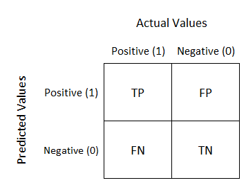
# Accuracy: Overall, how often is the classifier correct?
# (TP+TN)/total = (1136+1061)/(1136 + 229 + 279 + 1061)
(1136+1061)/(1136 + 229 + 279 + 1061)

0.8121996303142329

# Accuracy: Overall, how often is the classifier correct?
# (TP+TN)/total = (1116+1094)/(1136 + 229 + 279 + 1061)
(1116+1094)/(1136 + 229 + 279 + 1061)

0.8170055452865065