Solving Sudoku is so much fun, but how about training a machine that can solve sudoku at a rate of 150+ sudokus per minute? 😮

In this tutorial, I will show how easy it is to code your own sudoku solver using deep learning and some image processing.
-
OpenCV: OpenCV is a library of programming functions mainly aimed at real-time computer vision plus its open-source, fun to work with and my personal favorite. I have used version 4.1.0 for this project.
-
Python: aka swiss army knife of coding. I have used version 3.6.7 here.
-
IDE: I will be using Jupyter notebooks for this project.
-
Keras: Easy to use and widely supported, Keras makes deep learning about as simple as deep learning can be.
-
Scikit-Learn: It is a free software machine learning library for the Python programming language.
-
And of course, do not forget the coffee!
Let’s begin by creating a workspace.
Creating a workspace.
I recommend making a conda environment because it makes project management much easier. Please follow the instructions in this link for installing mini-conda. Once installed open cmd/terminal and create an environment using-
{% highlight bash linenos %}
conda create -n 'name_of_the_environment' python=3.6 {% endhighlight %}
Now let’s activate the environment:
{% highlight bash linenos %}
conda activate 'name_of_the_environment' {% endhighlight %}
This should set us inside our virtual environment. Time to install some libraries-
{% highlight bash linenos %}
# installing OpenCV
pip install opencv-python==4.1.0# Installing Keras
pip install keras# Installing Jupyter
pip install jupyter#Installing Scikit-Learn
pip install scikit-learn {% endhighlight %}
Finally, let’s open jupyter notebook using the below command and start coding.
{% highlight bash linenos %}
jupyter notebook {% endhighlight %}
To make this simple, I have divided the approach into 3 parts-
- Looking for sudoku in the image.
- Extracting numbers from sudoku.
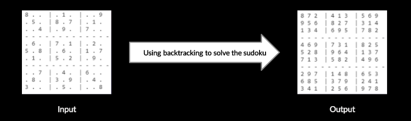
- Solving the Sudoku using backtracking.
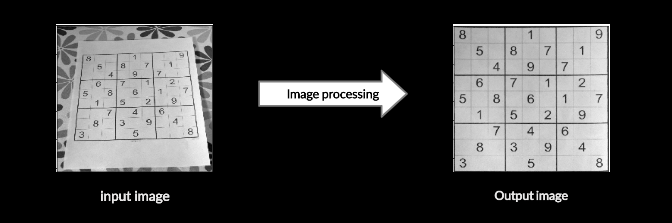
In this part, we’ll be focusing on how to extract the sudoku grid i.e. our Region of Interest (ROI) from the input image.

1. Converting the input image to a binary image: This step involves converting the input image to a greyscale image, applying gaussian blur to the grey-scale image, followed by thresholding, bitwise_not and dilating the image.
Grey-scale: Colored digital images are nothing but 3-dimensional arrays containing pixel data in the form of numbers. Ideally there are 3 channels: RGB (Red, Green, & Blue) and when we convert a colored image to greyscale, we just keep a single channel instead of 3 and this channel has a value ranging from 0–255 where 0 corresponds to a black pixel and 255corresponds to a white pixel and remaining values decide how gray the pixel is (the closer to 0, the darker it is).

Gaussian Blur: An image blurring technique in which the image is convolved with a Gaussian kernel. I’ll be using it to smoothen the input image by reducing noise.

Thresholding: In grayscaled images, each pixel has a value between 0–255, to convert such an image to a binary image we apply thresholding. To do this, we choose a threshold value between 0–255 and check each pixel’s value in the grayscale image. If the value is less than the threshold, it is given a value of 0 else 1.
In binary images, the pixels have just 2 values (0: Black, 1:White) and hence, it makes edge detection much easier.

{% highlight python linenos %}
def pre_process_image(img, skip_dilate=False):
"""Uses a blurring function, adaptive thresholding and dilation to expose the main features of an image."""
 # Gaussian blur with a kernal size (height, width) of 9.
 # Note that kernal sizes must be positive and odd and the kernel must be square.
 proc = cv2.GaussianBlur(img.copy(), (9, 9), 0)

 # Adaptive threshold using 11 nearest neighbour pixels
 proc = cv2.adaptiveThreshold(proc, 255, cv2.ADAPTIVE_THRESH_GAUSSIAN_C, cv2.THRESH_BINARY, 11, 2)

 # Invert colours, so gridlines have non-zero pixel values.
 # Necessary to dilate the image, otherwise will look like erosion instead.
 proc = cv2.bitwise_not(proc)

 if not skip_dilate:
     # Dilate the image to increase the size of the grid lines.
     kernel = np.array([[0., 1., 0.], [1., 1., 1.], [0., 1., 0.]], np.uint8)
     proc = cv2.dilate(proc, kernel)

 plt.imshow(proc, cmap='gray')
 plt.title('pre_process_image')
 plt.show()
 return proc
{% endhighlight %}
2. Detecting the largest polygon in the image: This step involves finding the contours from the previous image and selecting the largest contour (corresponds to the largest grid). Now from the largest contour, selecting the extreme most points and that would be the 4 corners. The function cv2.findContours returns all the contours it finds in the image. After sorting the returned contours from the image by area, the largest contour can easily be selected. And once we have the largest polygon, we can easily select the 4 corners (displayed as the 4 green points in the third image in figure 1).
- Contour detection: Contours can be explained simply as a curve joining all the continuous points (along the boundary), having the same color or intensity.

{% highlight python linenos %}
def find_corners_of_largest_polygon(img): """Finds the 4 extreme corners of the largest contour in the image.""" _, contours, h = cv2.findContours(img.copy(), cv2.RETR_EXTERNAL, cv2.CHAIN_APPROX_SIMPLE) # Find contours contours = sorted(contours, key=cv2.contourArea, reverse=True) # Sort by area, descending polygon = contours[0] # Largest image
# Use of `operator.itemgetter` with `max` and `min` allows us to get the index of the point
# Each point is an array of 1 coordinate, hence the [0] getter, then [0] or [1] used to get x and y respectively.

# Bottom-right point has the largest (x + y) value
# Top-left has point smallest (x + y) value
# Bottom-left point has smallest (x - y) value
# Top-right point has largest (x - y) value
bottom_right, _ = max(enumerate([pt[0][0] + pt[0][1] for pt in polygon]), key=operator.itemgetter(1))
top_left, _ = min(enumerate([pt[0][0] + pt[0][1] for pt in polygon]), key=operator.itemgetter(1))
bottom_left, _ = min(enumerate([pt[0][0] - pt[0][1] for pt in polygon]), key=operator.itemgetter(1))
top_right, _ = max(enumerate([pt[0][0] - pt[0][1] for pt in polygon]), key=operator.itemgetter(1))

# Return an array of all 4 points using the indices
# Each point is in its own array of one coordinate
return [polygon[top_left][0], polygon[top_right][0], polygon[bottom_right][0], polygon[bottom_left][0]]
{% endhighlight %}
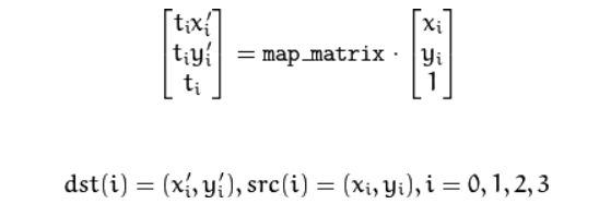
3. Cropping and warping the detected polygon: The approach is simple since we have the coordinates of the 4 corners, we can use this to crop and wrap the original image resulting in the final image in figure 1.
See the two images in the figure above? Both of them are cropped but still, the one on the right is much better than the one on the left. That’s because of warping, it gives a better perspective of the image. I’ll explain how we can achieve warping using cv2.warpPerspective() cv2.warpPerspective function takes 3 arguments source image (src), transformation matrix (m), and size of the destination image (size, size). transformation matrix. Now transformation matrix is a 3x3 matrix that helps us calculate the perspective transform. We can get the transformation matrix using cv2.getPerspectiveTransform(source_image, destination_image).

{% highlight python linenos %} def crop_and_warp(img, crop_rect): """Crops and warps a rectangular section from an image into a square of similar size."""
# Rectangle described by top left, top right, bottom right and bottom left points
top_left, top_right, bottom_right, bottom_left = crop_rect[0], crop_rect[1], crop_rect[2], crop_rect[3]

# Explicitly set the data type to float32 or `getPerspectiveTransform` will throw an error
src = np.array([top_left, top_right, bottom_right, bottom_left], dtype='float32')

# Get the longest side in the rectangle
side = max([
    distance_between(bottom_right, top_right),
    distance_between(top_left, bottom_left),
    distance_between(bottom_right, bottom_left),
    distance_between(top_left, top_right)
    ])

# Describe a square with side of the calculated length, this is the new perspective we want to warp to
dst = np.array([[0, 0], [side - 1, 0], [side - 1, side - 1], [0, side - 1]], dtype='float32')

# Gets the transformation matrix for skewing the image to fit a square by comparing the 4 before and after points
m = cv2.getPerspectiveTransform(src, dst)

# Performs the transformation on the original image
warp = cv2.warpPerspective(img, m, (int(side), int(side)))
plt.imshow(warp, cmap='gray')
plt.title('warp_image')
plt.show()
return warp
{% endhighlight %}

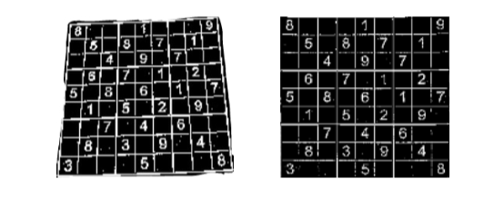
- Eliminating noise from the binary image: We’ll use a gaussian blur to remove the noise from the warped image resulting in a better image.
- Extracting the smaller grids: Since we already know that a sudoku grid has 81 similar dimensional cells (9 rows and 9 columns). We can simply iterate over the row length and column length of the image, check for points every 1/9th of the length of row/column distance apart and stored the set of pixels that were in between in an array. Some of the sample pixels extracted are shown in the last image in figure 2.
- Since we now have the individual grids that contain the digit information, we need to build a neural network that is capable of recognize the digits.
- Data: We should expect 10 types of characters, 1–9 and null i.e. blank space that is needed to be filled. I’ve created the data using the above-mentioned grid extraction method from different sudoku images. 30 samples for each digit.
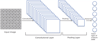
- CNN: The convolutional neural network that I’ve made is 6 layers deep (4 hidden layers) sequential model. To keep the model simple, we’ll start by creating a sequential object.
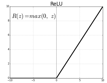
- The first layer will be a convolutional layer with 32 output filters, a convolution window of size (16, 16), and ‘ReLU’ as the activation function.

- Next, we’ll be adding a max-pooling layer with a window size of (2,2). Max pooling is a sample-based discretization process. The objective is to down-sample an input representation (image, hidden-layer output matrix, etc.), reducing its dimensionality and allowing for assumptions to be made about features contained in the sub-regions binned.


-
Now, we will be adding some dropout rate to take care of overfitting. Dropout is a regularization hyperparameter initialized to prevent Neural Networks from Overfitting. Dropout is a technique where randomly selected neurons are ignored during training. They are “dropped-out” randomly. We have chosen a dropout rate of 0.5 which means 50% of the nodes will be retained.
-
Now it’s time to flatten the node data so we add a flatten layer for that. The flatten layer takes data from the previous layer and represents it in a single dimension.

- Finally, we will be adding 2 dense layers, one with the dimensionality of the output space as 128, activation function=’relu’ and other, our final layer with 10 output classes for categorizing the 10 digits (0–9) and activation function=’ softmax’.
{% highlight python linenos %}
from keras.models import Sequential from keras.layers import Dense from keras.layers import Dropout from keras.layers import Flatten from keras.layers.convolutional import Conv2D, MaxPooling2D from sklearn.model_selection import train_test_split from keras.utils import np_utils
data = pd.read_csv('image_data.csv')
X = [] Y = data['y'] del data['y'] for i in range(data.shape[0]): flat_pixels = data.iloc[i].values[1:] image = np.reshape(flat_pixels, (28,28)) X.append(image)
X = np.array(X) Y = np.array(Y)
(X_train, X_test, Y_train, Y_test) = train_test_split(X, Y, test_size=0.30, random_state=42) y_test = Y_test.copy()
Y_train = np_utils.to_categorical(Y_train) Y_test = np_utils.to_categorical(Y_test)
#reshaping data X_train = X_train.reshape(-1,28,28,1) X_test = X_test.reshape(-1,28,28,1)
num_classes = 11
model_ = Sequential() model_.add(Conv2D(32, (16,16), input_shape=(28, 28, 1), activation='relu')) model_.add(MaxPooling2D(pool_size=(2, 2))) model_.add(Dropout(0.5)) model_.add(Flatten()) model_.add(Dense(128, activation='relu')) model_.add(Dense(units=num_classes, activation='softmax'))
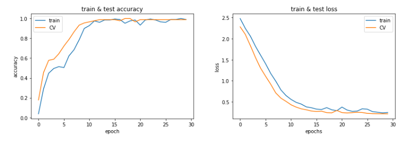
model_.compile(loss='categorical_crossentropy', optimizer='adam', metrics=['accuracy']) model_.fit(X_train, Y_train, validation_data=(X_test, Y_test), epochs=30, batch_size=200, verbose=2)
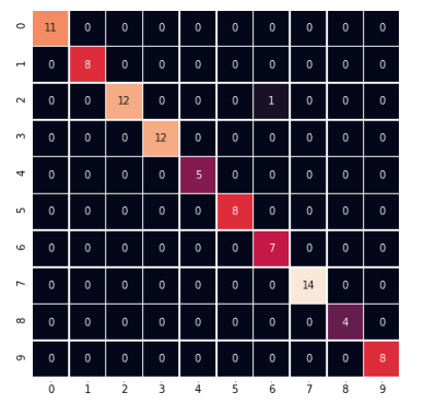
scores = model_.evaluate(X_test,Y_test, verbose=0) print("CNN Error: %.2f%%" % (100-scores[1]*100)) {% endhighlight %}
The dataset I have created is small but works well. It contains 30 sample images of size 28x28 for each of the digits (0–9). Here 0 corresponds to the blank space in sudoku. Now we need to split the data into 2 sets-
- Training data set: We use this data to train the model.
- Test data set: This data is unseen for the model so we will use this to test the performance of the created model on unseen data. The train test split is 70–30 i.e 30% of points are selected from the whole dataset randomly and assigned as the test set. The remaining 70% points are assigned as the train set.

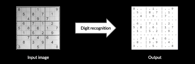
These are the prediction results from some of the sample grids that I extracted and as we can see the predictions are pretty accurate, we can proceed to the next step:
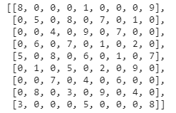
Detecting all the characters and storing them in an array of dimensions 9x9.
We traverse through all the grids that we extracted from the sudoku and get the predicted character from our model we’ll end up with an array-
- Note: here 0 corresponds to the blank space.
Now that we have converted the image into an array, we just need to make a function that can fill up the blank spaces effectively given the rules of sudoku. I found backtracking very efficient at this so let’s talk more about it.
Backtracking is an algorithmic-technique for solving problems recursively by trying to build a solution incrementally, one piece at a time, removing those solutions that fail to satisfy the constraints of the problem at any point.

Let’s understand how backtracking works through an example using a 3x3 sudoku. Suppose we’ve to solve the grid given the constraints-
-
Each column has unique numbers from 1 to ’n’ or empty spaces.
-
Each column has unique numbers from 1 to ’n’ or empty spaces.
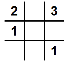


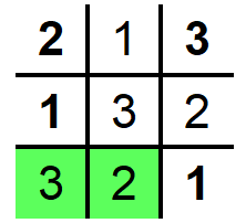
1. We need to fill 5 spaces, let’s start by iterating over the blank spaces from left to right and top to bottom.
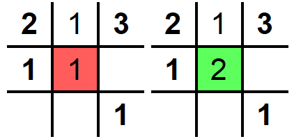
2. Let’s put 1 in the first encountered space and check if all the constraints are satisfied. Seems 1 is good here as it is unique in its row and column.
3. Moving on to the next grid, we again start by keeping 1 but as we can see that it is not unique in the column so we check for 2 and 2 satisfies all the constraints
4. For the 3rd empty grid, we can see none of the 3 numbers 1,2,3 satisfy the constraints.
5. To fix this, we take a step back and increment the number in the last grid we filled and make sure that the constraints are satisfied. Now we proceed with the next grig again and we can see that 2 fits in it.
6. Similarly, we fill the remaining grids and reach the optimal solution.
Now that we’ve understood how backtracking works, let’s make a function using the constraints used while solving a 9x9 sudoku and test it on the array we obtained from the previous step.
{% highlight python linenos %}
def find_empty_grid(x): # checks for empty spaces '0'. for i in range(len(x)): for j in range(len(x[0])): if x[i][j] == 0: return (i, j) #return row, col
return None
def solve_array(x): find = find_empty_grid(x) #find the empty spaces if not find: return True else: row, col = find
for i in range(1,10):
    if valid(x, i, (row, col)): #check the constraints
        x[row][col] = i

        if solve_array(x):
            return True

        x[row][col] = 0

return False
def valid(x, num, pos): #this function checks the constraints # Check row for i in range(len(x[0])): if x[pos[0]][i] == num and pos[1] != i: return False
# Check column
for i in range(len(x)):
    if x[i][pos[1]] == num and pos[0] != i:
        return False

# Check box
box_x = pos[1] // 3
box_y = pos[0] // 3

for i in range(box_y*3, box_y*3 + 3):
    for j in range(box_x * 3, box_x*3 + 3):
        if x[i][j] == num and (i,j) != pos:
            return False

return True
def print_board(x): #this function is for printing the array with a better look for i in range(len(x)): if i % 3 == 0 and i != 0: print("- - - - - - - - - - - - - ")
    for j in range(len(x[0])):
        if j % 3 == 0 and j != 0:
            print(" | ", end="")

        if j == 8:
            k = '.' if x[i][j]==0 else str(x[i][j])
            print(k)
        else:
            k = '.' if x[i][j]==0 else str(x[i][j])
            print(k + " ", end="")
{% endhighlight %}

Final comment
Thank you for reading the blog, hope this project is useful for some of you aspiring to do projects on OCR, image processing, Machine Learning, IoT.
And if you have any doubts regarding this project, please leave a comment in the response section.
Kaggle notebook link: https://www.kaggle.com/sarthakvajpayee/simple-ai-sudoku-solver?scriptVersionId=40346804
Github repo link: https://github.com/SarthakV7/ai_sudoku_solver
Find me on LinkedIn: www.linkedin.com/in/sarthak-vajpayee