Hands-on Transformers (Kaggle Google QUEST Q&A Labeling).
Part 3/3 of Transformers vs Google QUEST Q&A Labeling (Kaggle top 5%).

This is a 3 part series where we will be going through Transformers, BERT, and a hands-on Kaggle challenge — Google QUEST Q&A Labeling to see Transformers in action (top 4.4% on the leaderboard). In this part (3/3) we will be looking at a hands-on project from Google on Kaggle. Since this is an NLP challenge, I’ve used transformers in this project. I have not covered transformers in much detail in this part but if you wish you could check out the part 1/3 of this series where I’ve discussed transformers in detail.
Bird's eye view of the blog:
To make the reading easy, I’ve divided the blog into different sub-topics-
-
Problem statement and evaluation metrics.
-
About the data.
-
Exploratory Data Analysis (EDA).
-
Modeling (includes data preprocessing).
-
Post-modeling analysis.
Problem statement and Evaluation metrics:
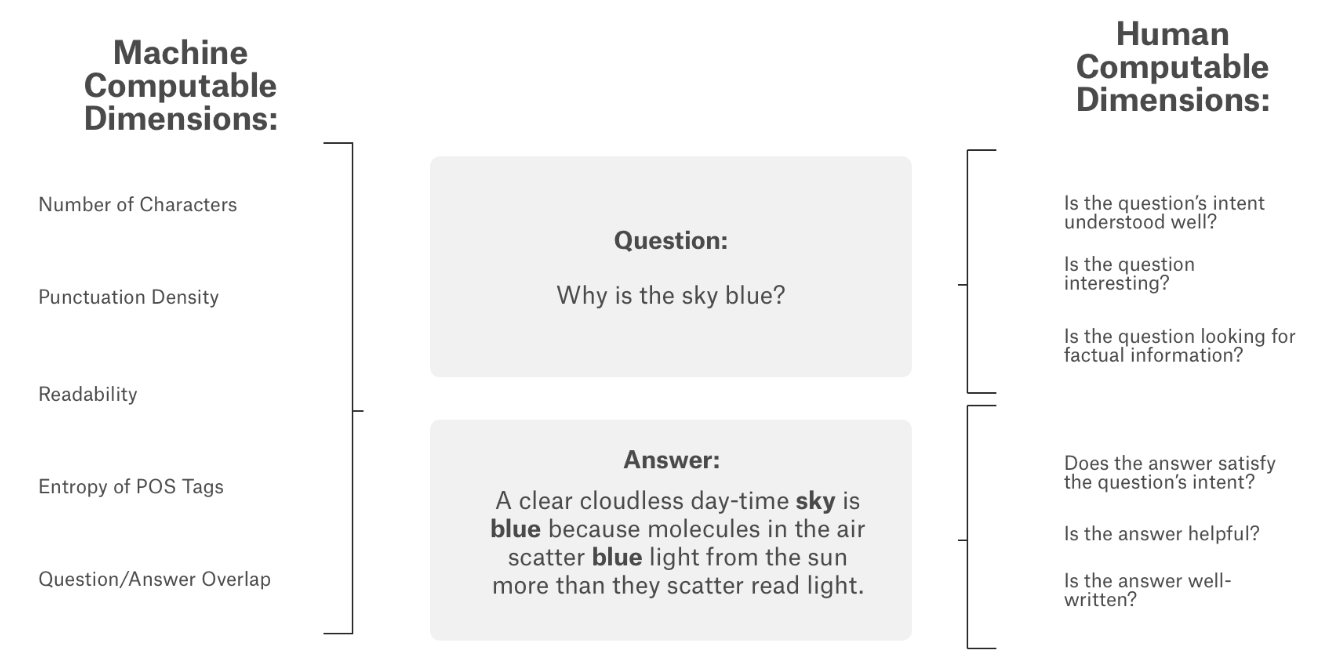
Computers are really good at answering questions with single, verifiable answers. But, humans are often still better at answering questions about opinions, recommendations, or personal experiences.
Humans are better at addressing subjective questions that require a deeper, multidimensional understanding of context. Questions can take many forms — some have multi-sentence elaborations, others may be simple curiosity or a fully developed problem. They can have multiple intents, or seek advice and opinions. Some may be helpful and others interesting. Some are simple right or wrong.
Unfortunately, it’s hard to build better subjective question-answering algorithms because of a lack of data and predictive models. That’s why the CrowdSource team at Google Research, a group dedicated to advancing NLP and other types of ML science via crowdsourcing, has collected data on a number of these quality scoring aspects.
In this competition, we’re challenged to use this new dataset to build predictive algorithms for different subjective aspects of question-answering. The question-answer pairs were gathered from nearly 70 different websites, in a “common-sense” fashion. The raters received minimal guidance and training and relied largely on their subjective interpretation of the prompts. As such, each prompt was crafted in the most intuitive fashion so that raters could simply use their common-sense to complete the task.
Demonstrating these subjective labels can be predicted reliably can shine a new light on this research area. Results from this competition will inform the way future intelligent Q&A systems will get built, hopefully contributing to them becoming more human-like.
Evaluation metric: Submissions are evaluated on the mean column-wise Spearman’s correlation coefficient. The Spearman’s rank correlation is computed for each target column, and the mean of these values is calculated for the submission score.
About the data:
The data for this competition includes questions and answers from various StackExchange properties. Our task is to predict the target values of 30 labels for each question-answer pair. The list of 30 target labels is the same as the column names in the sample_submission.csv file. Target labels with the prefix question_ relate to the question_title and/or question_body features in the data. Target labels with the prefix answer_ relate to the answer feature. Each row contains a single question and a single answer to that question, along with additional features. The training data contains rows with some duplicated questions (but with different answers). The test data does not contain any duplicated questions. Target labels can have continuous values in the range [0,1]. Therefore, predictions must also be in that range. The files provided are:
-
train.csv — the training data (target labels are the last 30 columns)
-
test.csv — the test set (you must predict 30 labels for each test set row)
-
sample_submission.csv — a sample submission file in the correct format; column names are the 30 target labels
You can check out the dataset using this link.
Exploratory Data Analysis (EDA)
Check-out the notebook with in-depth EDA + Data Scraping (Kaggle link).
The training data contains 6079 listings and each listing has 41 columns. Out of these 41 columns, the first 11 columns/features have to be used as the input and the last 30 columns/features are the target predictions. Let’s take a look at the input and target labels:

The output features are all of the float types between 0 and 1.
Let's explore the input labels one by one.
qa_id
Question answer ID represents the id of a particular data point in the given dataset. Each data point has a unique qa_id. This feature is not to be used for training and will be used later while submitting the output to Kaggle.

question_title
This is a string data type feature that holds the title of the question asked. For the analysis of question_title, I’ll be plotting a histogram of the number of words in this feature.
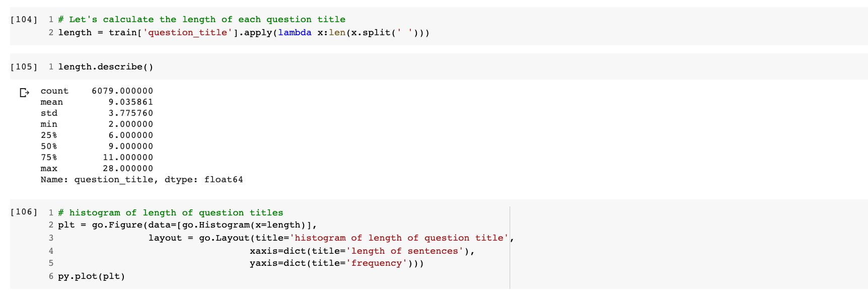

From the analysis, it is evident that:
- Most of the question_title features have a word length of around 9.
- The minimum question length is 2.
- The maximum question length is 28.
- 50% of question_title have lengths between 6 and 11.
- 25% of question_title have lengths between 2 and 6.
- 25% of question_title have lengths between 11 and 28.
question_body
This is again a string data type feature that holds the detailed text of the question asked. For the analysis of question_body, I’ll be plotting a histogram of the number of words in this feature.
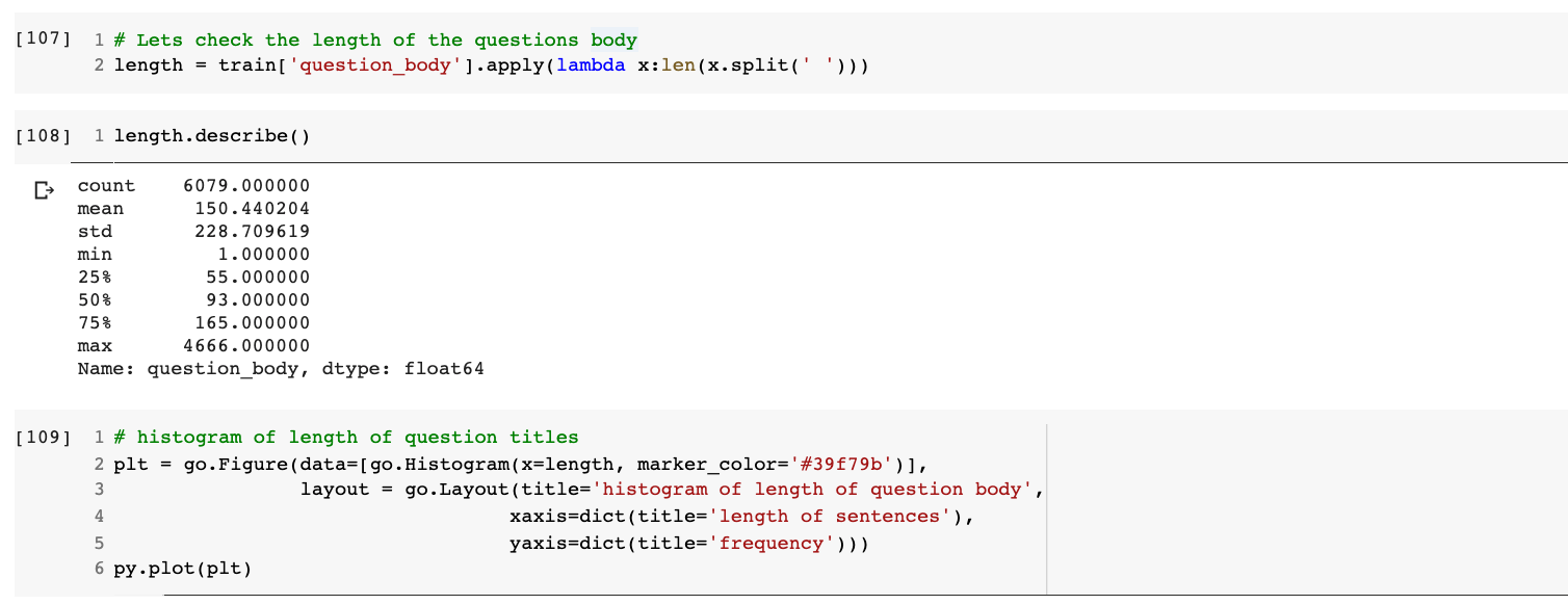

From the analysis, it is evident that:
- Most of the question_body features have a word length of around 93.
- The minimum question length is 1.
- The maximum question length is 4666.
- 50% of question_title have lengths between 55 and 165.
- 25% of question_title have lengths between 1 and 55.
- 25% of question_title have lengths between 165 and 4666.
The distribution looks like a power-law distribution, it can be converted to a gaussian distribution using log and then used as an engineered feature.
question_user_name
This is a string data type feature that denotes the name of the user who asked the question. For the analysis of question_answer, I’ll be plotting a histogram of the number of words in this feature.
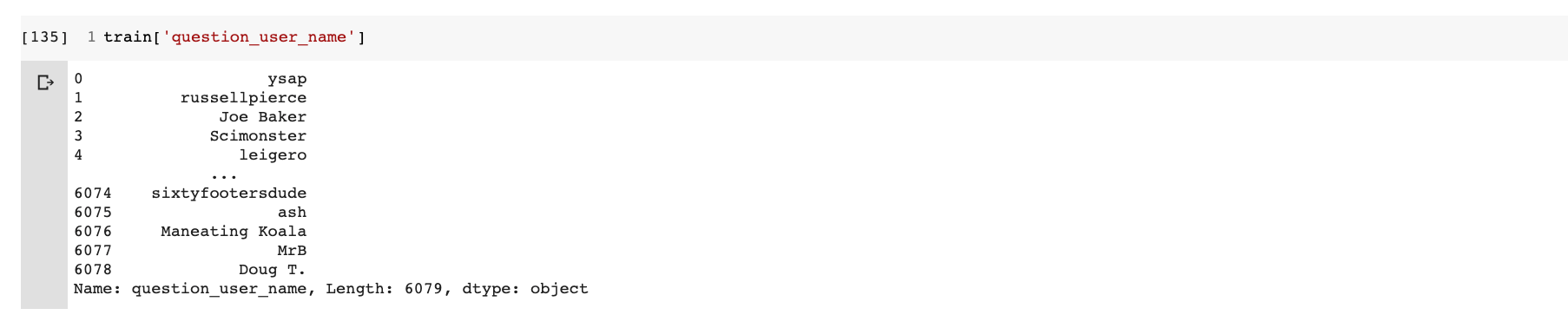
I did not find this feature of much use therefore I won’t be using this for modeling.
question_user_page
This is a string data type feature that holds the URL to the profile page of the user who asked the question.

On the profile page, I noticed 4 useful features that could be used and should possibly contribute to good predictions. The features are:
- Reputation: Denotes the reputation of the user.
- gold_score: The number of gold medals awarded.
- silver_score: The number of silver medals awarded.
- bronze_score: The number of bronze medals awarded.
answer
This is again a string data type feature that holds the detailed text of the answer to the question. For the analysis of answer, I’ll be plotting a histogram of the number of words in this feature.
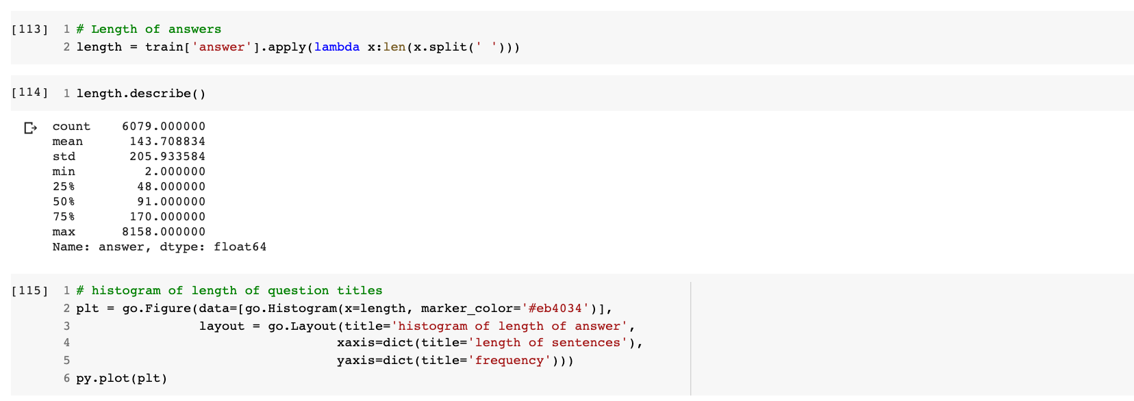
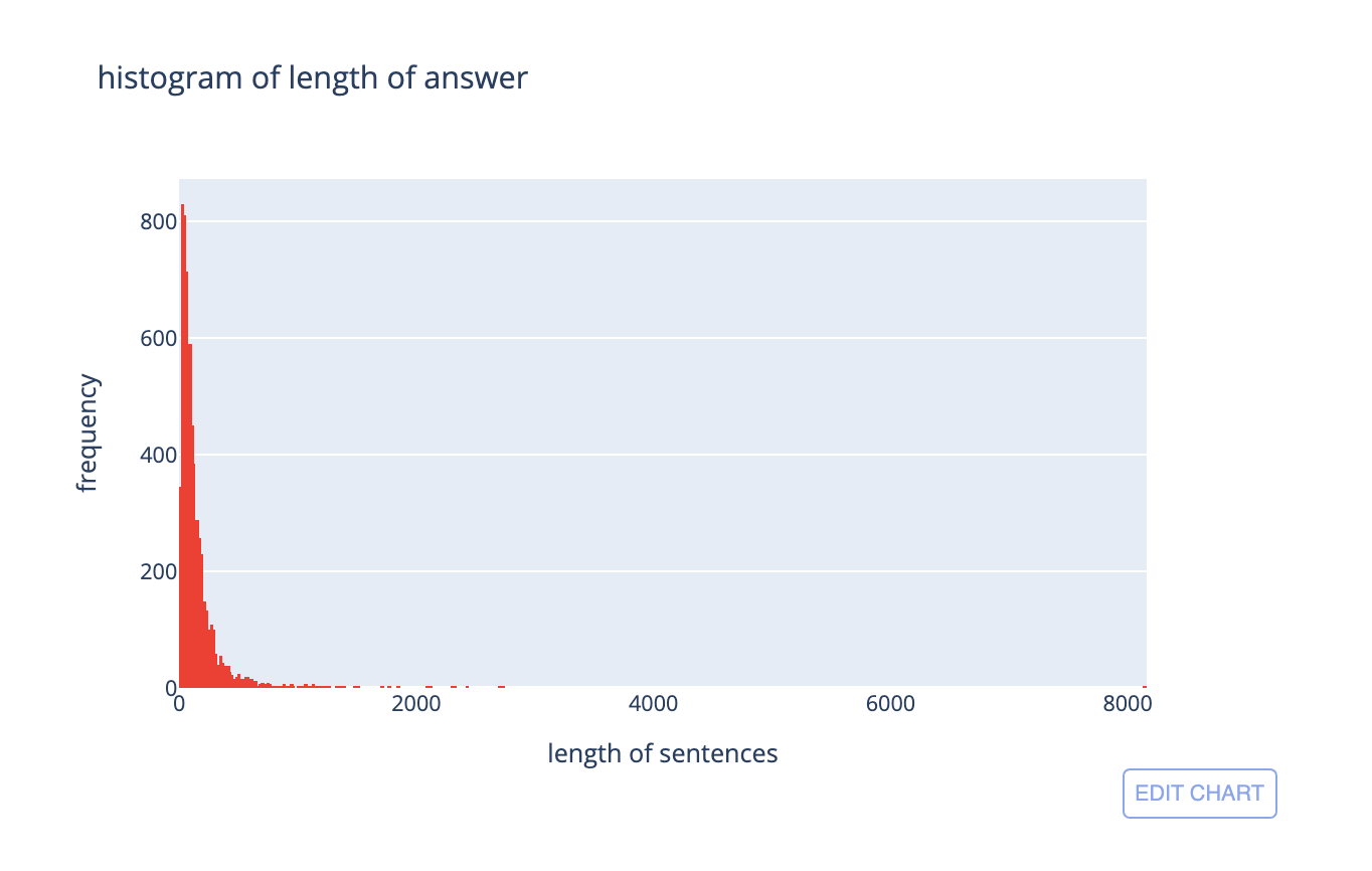
From the analysis, it is evident that:
- Most of the question_body features have a word length of around 143.
- The minimum question length is 2.
- The maximum question length is 8158.
- 50% of question_title have lengths between 48 and 170.
- 25% of question_title have lengths between 2 and 48.
- 25% of question_title have lengths between 170 and 8158.
This distribution also looks like a power-law distribution, it can also be converted to a gaussian distribution using log and then used as an engineered feature.
answer_user_name
This is a string data type feature that denotes the name of the user who answered the question.
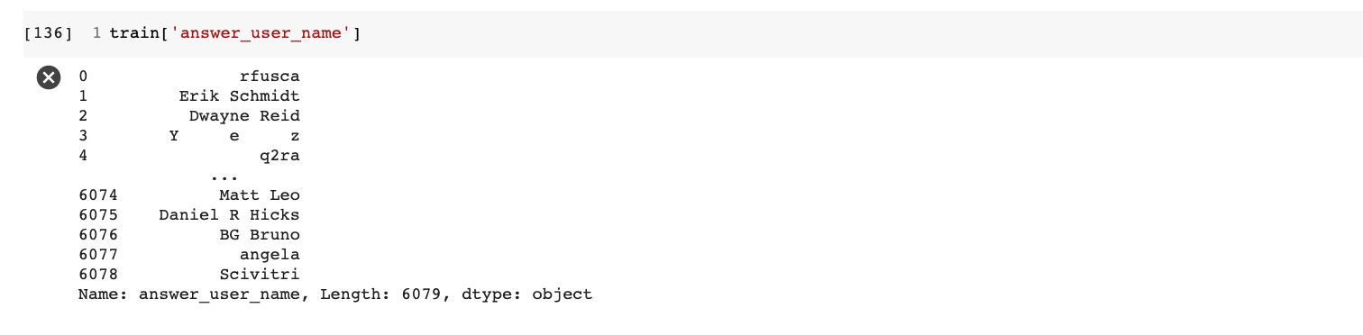
I did not find this feature of much use therefore I won’t be using this for modeling.
answer_user_page
This is a string data type feature similar to the feature “question_user_page” that holds the URL to the profile page of the user who asked the question.
I also used the URL in this feature to scrape the external data from the user’s profile page, similar to what I did for the feature ‘question_user_page’.
url
This feature holds the URL of the question and answers page on StackExchange or StackOverflow. Below I’ve printed the first 10 url data-points from train.csv
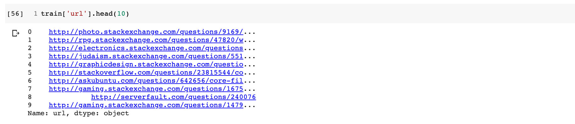
One thing to notice is that this feature lands us on the question-answer page, and that page may usually contain a lot more data like comments, upvotes, other answers, etc. which can be used for generating more features if the model does not perform well due to fewer data in train.csv Let’s see the data is present and what additional data can be scraped from the question-answer page.
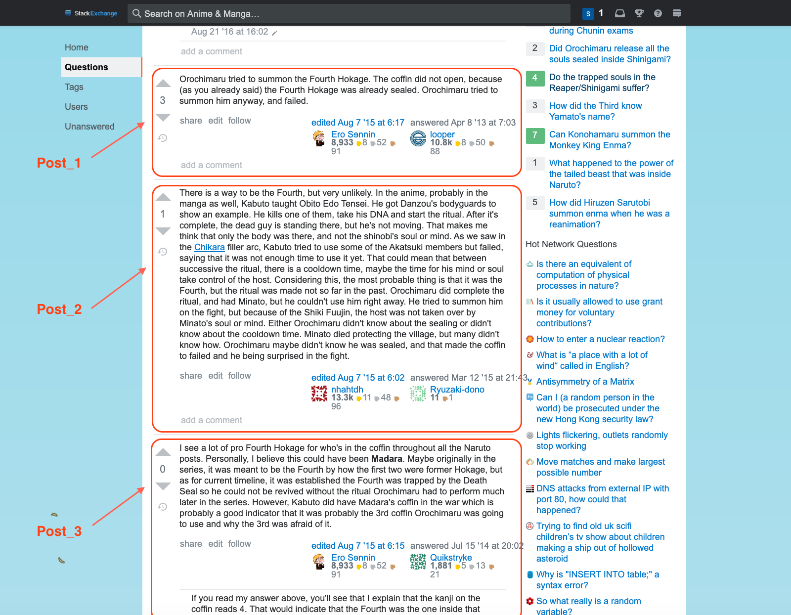
In the snapshot attached above, Post 1 and Post 2 contain the answers, upvotes, and comments for the question asked in decreasing order of upvotes. The post with a green tick is the one containing the answer provided in the train.csv file.
Each question may have more than one answer. We can scrape these answers and use them as additional data.

The snapshot above defines the anatomy of a post. We can scrape useful features like upvotes and comments and use them as additional data.
Below is the code for scraping the data from the URL page.
<iframe src="https://medium.com/media/1fa6c4f98d68f1f87bd5b29919b0e760" frameborder=0></iframe>There are 8 new features that I’ve scraped-
- upvotes: The number of upvotes on the provided answer.
- comments_0: Comments to the provided answer.
- answer_1: Most voted answer apart from the one provided.
- comment_1: Top comment to answer_1.
- answer_2: Second most voted answer.
- comment_2: Top comment to answer_2.
- answer_3: Third most voted answer.
- comment_3: Top comment to answer_3.
category
This is a categorical feature that tells the categories of question and answers pairs. Below I’ve printed the first 10 category data-points from train.csv

Below is the code for plotting a Pie chart of category.
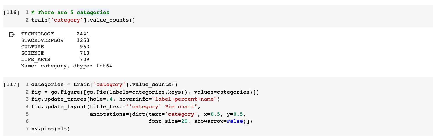
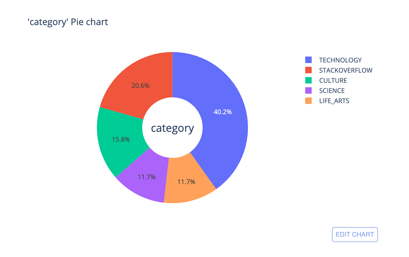
The chart tells us that most of the points belong to the category *TECHNOLOGY *and least belong to *LIFE_ARTS *(709 out of 6079).
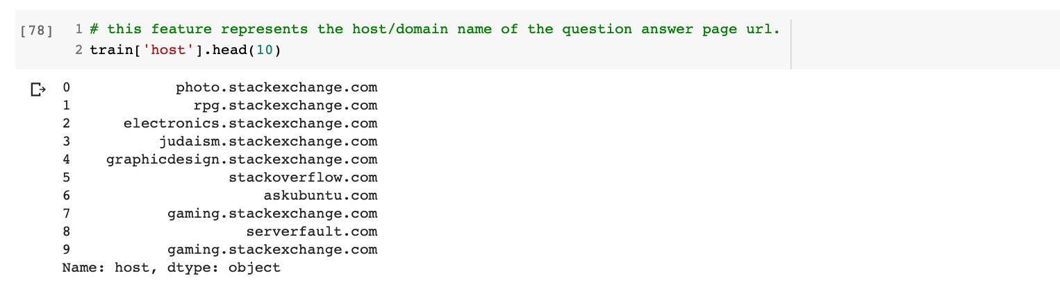
host
This feature holds the host or domain of the question and answers page on StackExchange or StackOverflow. Below I’ve printed the first 10 host data-points from train.csv
Below is the code for plotting a bar graph of unique hosts.
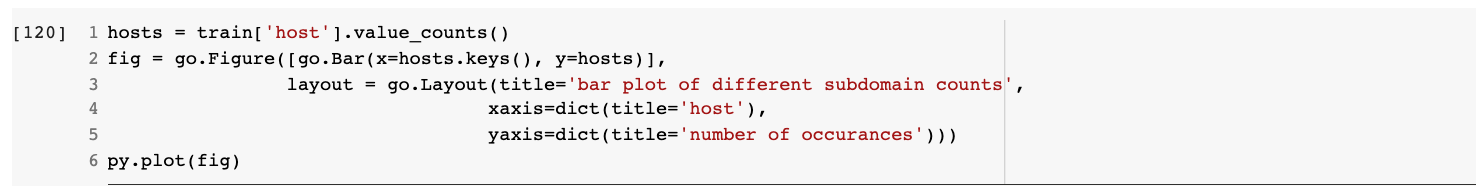

It seems there are not many but just 63 different subdomains present in the training data. Most of the data points are from StackOverflow.com whereas least from meta.math.stackexchange.com
Target values
Let’s analyze the target values that we need to predict. But first, for the sake of a better interpretation, please check out the full dataset on kaggle using this link.
Below is the code block displaying the statistical description of the target values. These are only the first 6 features out of all the 30 features. The values of all the features are of type float and are between 0 and 1.

Notice the second code block which displays the unique values present in the dataset. There are just 25 unique values between 0 and 1. This could be useful later while fine-tuning the code.
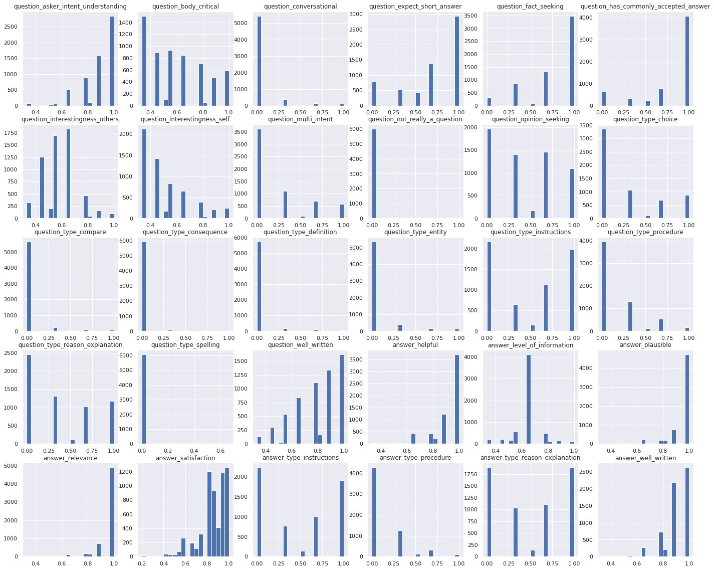
Finally, let’s check the distribution of the target features and their correlation.


Modeling

Now that we know our data better through EDA, let’s begin with modeling. Below are the subtopics that we’ll go through in this section-
-
Overview of the architecture: Quick rundown of the ensemble architecture and it’s different components.
-
Base learners: Overview of the base learners used in the ensemble.
-
Preparing the data: Data cleaning and preparation for modeling.
-
Ensembling: Creating models for training, and predicting. Pipelining the data preparation, model training, and model prediction steps.
-
**Getting the scores from Kaggle: **Submitting the predicted target values for test data on Kaggle and generating a leaderboard score to see how well the ensemble did.
I tried various deep neural network architectures with GRU, Conv1D, Dense layers, and with different features for the competition but, an ensemble of 8 transformers (as shown above) seems to work the best. In this part, we will be focusing on the final architecture of the ensemble used and for the other baseline models that I experimented with, you can check out my github repo.
Overview of the architecture:
Remember our task was for a given *question_title, question_body, and answer, *we had to predict 30 target labels. Now out of these 30 target labels, the first 21 are related to the question_title and question_body and have no connection to the answer whereas the last 9 target labels are related to the answer only but out of these 9, some of them also take question_title and question_body into the picture. Eg. features like answer_relevance and answer_satisfaction can only be rated by looking at both the question and answer.

With some experimentation, I found that the base-learner (BERT_base) performs exceptionally well in predicting the first 21 target features (related to questions only) but does not perform that well in predicting the last 9 target features. Taking note of this, I constructed 3 dedicated base-learners and 2 different datasets to train them.
-
The first base-learner was dedicated to predicting the question-related features (first 21) only. The dataset used for training this model consisted of features question_title and question_body only.
-
The second base-learner was dedicated to predicting the answer-related features (last 9) only. The dataset used for training this model consisted of features question_title, question_body, and answer.
-
The third base-learner was dedicated to predicting all the 30 features. The dataset used for training this model again consisted of features question_title, question_body, and answer.
To make the architecture even more robust, I used 3 different types of base learners — BERT, RoBERTa, and XLNet. We will be going through these different transformer models later in this blog.
In the ensemble diagram above, we can see —
-
The 2 datasets consisting of [question_title + question_body] and **[question_title + question_body + answer] **being used separately to train different base learners.
-
Then we can see the 3 different base learners (BERT, RoBERTa, and XLNet) dedicated to predicting the question-related features only (first 21) colored in blue, using the dataset [question_title + question_body]
-
Next, we can see the 3 different base learners (BERT, RoBERTa, and XLNet) dedicated to predicting the answer-related features only (last 9) colored in green, using the dataset [question_title + question_body + answer].
-
Finally, we can see the 2 different base learners (BERT, and RoBERTa) dedicated to predicting all the 30 features colored in red, using the dataset [question_title + question_body + answer].
In the next step, the predicted data from models dedicated to predicting the **question-related features only **(denoted as bert_pred_q, roberta_pred_q, xlnet_pred_q) ****and the predicted data from ****models dedicated to predicting the **answer-related features only **(denoted as bert_pred_a, roberta_pred_a, xlnet_pred_a) is collected and concatenated column-wise which leads to a predicted data with all the 30 features. These concatenated features are denoted as xlnet_concat, roberta_concat, and bert_concat.
Similarly, the predicted data from ****models dedicated to predicting **all the 30 features **(denoted as bert_qa, roberta_qa) is collected. Notice that I’ve not used the XLNet model here for predicting all the 30 features because the scores were not up to the mark.
Finally, after collecting all the different predicted data — ***[xlnet_concat, roberta_concat, bert_concat, bert_qa, and roberta_qa], ***the final value is calculated by taking the average of all the different predicted values.
Base learners
Now we will take a look at the 3 different transformer models that were used as base learners.
- bert_base_uncased:
Bert was proposed by Google AI in late 2018 and since then it has become state-of-the-art for a wide spectrum of NLP tasks. It uses an architecture derived from transformers pre-trained over a lot of unlabeled text data to learn a language representation that can be used to fine-tune for specific machine learning tasks. BERT outperformed the NLP state-of-the-art on several challenging tasks. This performance of BERT can be ascribed to the transformer’s encoder architecture, unconventional training methodology like the Masked Language Model (MLM), and Next Sentence Prediction (NSP) and the humungous amount of text data (all of Wikipedia and book corpus) that it is trained on. BERT comes in different sizes but for this challenge, I’ve used bert_base_uncased.

The architecture of bert_base_uncased consists of 12 encoder cells with 8 attention heads in each encoder cell. It takes an input of size 512 and returns 2 values by default, the output corresponding to the first input token [CLS] which has a dimension of 786 and another output corresponding to all the 512 input tokens which have a dimension of (512, 768) aka pooled_output. But apart from these, we can also access the hidden states returned by each of the 12 encoder cells by passing ***output_hidden_states=True ***as one of the parameters. BERT accepts several sets of input, for this challenge, the input I’ll be using will be of 3 types:
-
*input_ids: *The token embeddings are numerical representations of words in the input sentence. There is also something called sub-word tokenization that BERT uses to first breakdown larger or complex words into simple words and then convert them into tokens. For example, in the above diagram look how the word ‘playing’ was broken into ‘play’ and ‘##ing’ before generating the token embeddings. This tweak in tokenization works wonders as it utilized the sub-word context of a complex word instead of just treating it like a new word.
-
*attention_mask: *The segment embeddings are used to help BERT distinguish between the different sentences in a single input. The elements of this embedding vector are all the same for the words from the same sentence and the value changes if the sentence is different. Let’s consider an example: Suppose we want to pass the two sentences “I have a pen” and *“The pen is red” *to BERT. The tokenizer will first tokenize these sentences as: **[‘[CLS]’, ‘I’, ‘have’, ‘a’, ‘pen’, ‘[SEP]’, ‘the’, ‘pen’, ‘is’, ‘red’, ‘[SEP]’] **And the segment embeddings for these will look like: **[0, 0, 0, 0, 0, 0, 1, 1, 1, 1, 1] **Notice how all the elements corresponding to the word in the first sentence have the same element 0 whereas all the elements corresponding to the word in the second sentence have the same element 1.
-
token_type_ids: The mask tokens that help BERT to understand what all input words are relevant and what all are just there for padding. Since BERT takes a 512-dimensional input, and suppose we have an input of 10 words only. To make the tokenized words compatible with the input size, we will add padding of size 512–10=502 at the end. Along with the padding, we will generate a mask token of size 512 in which the index corresponding to the relevant words will have 1s and the index corresponding to padding will have 0s.
2. XLNet_base_cased:
XLNet was proposed by Google AI Brain team and researchers at CMU in mid-2019. Its architecture is larger than BERT and uses an improved methodology for training. It is trained on larger data and shows better performance than BERT in many language tasks. The conceptual difference between **BERT **and XLNet is that while training BERT, the words are predicted in an order such that the previous predicted word contributes to the prediction of the next word whereas, XLNet learns to predict the words in an arbitrary order but in an autoregressive manner (not necessarily left-to-right).

This helps the model to learn bidirectional relationships and therefore better handles dependencies and relations between words. In addition to the training methodology, XLNet uses Transformer XL based architecture and 2 main key ideas: relative positional embeddings and the recurrence mechanism which showed good performance even in the absence of permutation-based training. XLNet was trained with over 130 GB of textual data and 512 TPU chips running for 2.5 days, both of which are much larger than BERT.
For XLNet, I’ll be using only **input_ids **and **attention_mask **as input.
3. RoBERTa_base:
RoBERTa was proposed by Facebook in mid-2019. It is a robustly optimized method for pretraining natural language processing (NLP) systems that improve on BERT’s self-supervised method. RoBERTa builds on BERT’s language masking strategy, wherein the system learns to predict intentionally hidden sections of text within otherwise unannotated language examples. RoBERTa modifies key hyperparameters in BERT, including removing BERT’s Next Sentence Prediction (NSP) objective, and training with much larger mini-batches and learning rates. This allows RoBERTa to improve on the masked language modeling objective compared with BERT and leads to better downstream task performance. RoBERTa was also trained on more data than BERT and for a longer amount of time. The dataset used was from existing unannotated NLP data sets as well as CC-News, a novel set drawn from public news articles.
For RoBERTa_base, I’ll be using only **input_ids **and **attention_mask **as input.
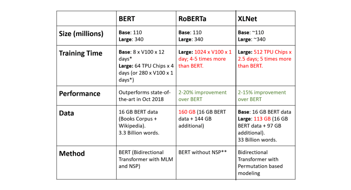
Finally here is the comparison of BERT, XLNet, and RoBERTa:

Preparing the data
Now that we have gained some idea about the architecture let’s see how to prepare the data for the base learners.
- As a preprocessing step, I have just treated the HTML syntax present in the features. I used html.unescape() to extract the text from HTML DOM elements. In the code snippet below, the function get_data() reads the train and test data and applies the preprocessing to the features question_title, question_body, and answer.
- The next step was to create input_ids, attention_masks, and token_type_ids from the input sentence. In the code snippet below, the function get_tokenizer() collects pre-trained tokenizer for the different base_learners. The second function fix_length() goes through the generated question tokens and answer tokens and makes sure that the maximum number of tokens is 512. The steps for fixing the number of tokens are as follows:
- If the input sentence has the number of tokens > 512, the sentence is trimmed down to 512.
- To trim the number of tokens, 256 tokens from the beginning and 256 tokens from the end are kept and the remaining tokens are dropped.
- For example, suppose an answer has 700 tokens, to trim this down to 512, 256 tokens from the beginning are taken and 256 tokens from the end are taken and concatenated to make 512 tokens. The remaining [700-(256+256) = 288] tokens that are in the middle of the answer are dropped.
- The logic makes sense because in a large text, the beginning part usually describes what the text is all about and the end part describes the conclusion of the text.
Next is the code block for generating the **input_ids, attention_masks, **and **token_type_ids. **I’ve used a condition that checks if the function needs to return the generated data for base learners relying on the dataset [question_title + question_body] or the dataset [question_title + question_body + answer].
<iframe src="https://medium.com/media/88dae21e444f9b86bf1bb91cd2269757" frameborder=0></iframe>Finally, here is the function that makes use of the function initialized above and generates **input_ids, attention_masks, **and **token_type_ids **for each of the instances in the provided data.
<iframe src="https://medium.com/media/c60fc558acd03defe75bcdc438194b1e" frameborder=0></iframe>To make the model training easy, I also created a class that generates train and cross-validation data based on the fold while using KFlod CV with the help of the functions specified above.
<iframe src="https://medium.com/media/3d1976731d01cbc79233ab9d5a2afa7e" frameborder=0></iframe> > **Ensembling**After data preprocessing, let's create the model architecture starting with base learners.
The code below takes the model name as input, collects the pre-trained model, and its configuration information according to the input name and creates the base learner model. Notice that output_hidden_states=True is passed after adding the config data.
<iframe src="https://medium.com/media/8ca36517206f8d715de8ffeb97c156cf" frameborder=0></iframe>The next code block is to create the ensemble architecture. The function accepts 2 parameters name that expects the name of the model that we want to train and model_type that expects the type of model we want to train. The model type can be **bert-base-uncased, roberta-base **or **xlnet-base-cased **whereas the model type can be **questions, answers, **or **question_answers. **The function create_model() takes the model_name and model_type and generates a model that can be trained on the specified data accordingly.
<iframe src="https://medium.com/media/6929a7ef4a7d8c69df6cfaac344c0382" frameborder=0></iframe>Now let's create a function for calculating the evaluation metric Spearman’s correlation coefficient.
<iframe src="https://medium.com/media/7cf04817683f11d2a934498844484f36" frameborder=0></iframe>Now we need a function that can collect the base learner model, data according to the base learner model, and train the model. I’ve used K-Fold cross-validation with 5 folds for training.
<iframe src="https://medium.com/media/b1c81ee6e1198036dba2f87945b1cb9a" frameborder=0></iframe>Now once we have trained the models and generated the predicted values, we need a function for calculating the weighted average. Here’s the code for that. *The weight’s in the weighted average are all 1s.
<iframe src="https://medium.com/media/11241d9afae12690989b978eb6007949" frameborder=0></iframe>Before bringing everything together, there is one more function that I used for processing the final predicted values. Remember in the EDA section there was an analysis of the target values where we noticed that the target values were only 25 unique floats between 0 and 1. To make use of that information, I calculated 61 (a hyperparameter) uniformly distributed percentile values and mapped them to the 25 unique values. This created 61 bins uniformly spaced between the upper and lower range of the target values. Now to process the predicted data, I used those bins to collect the predicted values and put them in the right place/order. This trick helped in improving the score in the final submission to the leaderboard to some extent.
<iframe src="https://medium.com/media/67fd8f961cb25e1729cbd67a5a527d87" frameborder=0></iframe>Finally, to bring the data-preprocessing, model training, and post-processing together, I created the get_predictions() function that-
- Collects the data.
- Creates the 8 base_learners.
- Prepares the data for the base_learners.
- Trains the base learners and collects the predicted values from them.
- Calculates the weighted average of the predicted values.
- Processes the weighted average prediction.
- Converts the final predicted values into a dataframe format requested by Kaggle for submission and return it.
Once the code compiles and runs successfully, it generates an output file that can be submitted to Kaggle for score calculation. The ranking of the code on the leaderboard is generated using the **score. **The ensemble model got a public score of **0.43658 **which makes it in the top 4.4% on the leaderboard.
Post modeling Analysis
Check-out the notebook with complete post-modeling analysis (Kaggle link).

Its time for some post-modeling analysis!
In this section, we will go through an analysis of train data to figure out what parts of the data is the model doing well on and what parts of the data it’s not. The main idea behind this step is to know the capability of the trained model and it works like a charm if applied properly for fine-tuning the model and data. But we won’t get into the fine-tuning part in this section, we will just be performing some basic EDA on the train data using the predicted target values for the train data. I’ll be covering the data feature by feature. Here are the top features we’ll be performing analysis on-
-
question_title, question_body, and answer.
-
Word lengths of question_title, question_body, and answer.
-
Host
-
Category
First, we will have to divide the data into a spectrum of good data and bad data. Good data will be the data points on which the model achieves a good score and bad data will be the data points on which the model achieves a bad score. Now for scoring, we will be comparing the actual target values of the train data with the model’s predicted target values on train data. I used mean squared error (MSE) as a metric for scoring since it focuses on how close the actual and target values are. Remember the more the MSE-score is, the bad the data point will be. Calculating the MSE-score is pretty simple. Here’s the code:
# Generating the MSE-score for each data point in train data.
from sklearn.metrics import mean_squared_error

train_score = [mean_squared_error(i,j) for i,j in zip(y_pred, y_true)]

# sorting the losses from minimum to maximum index wise.
train_score_args = np.argsort(train_score)
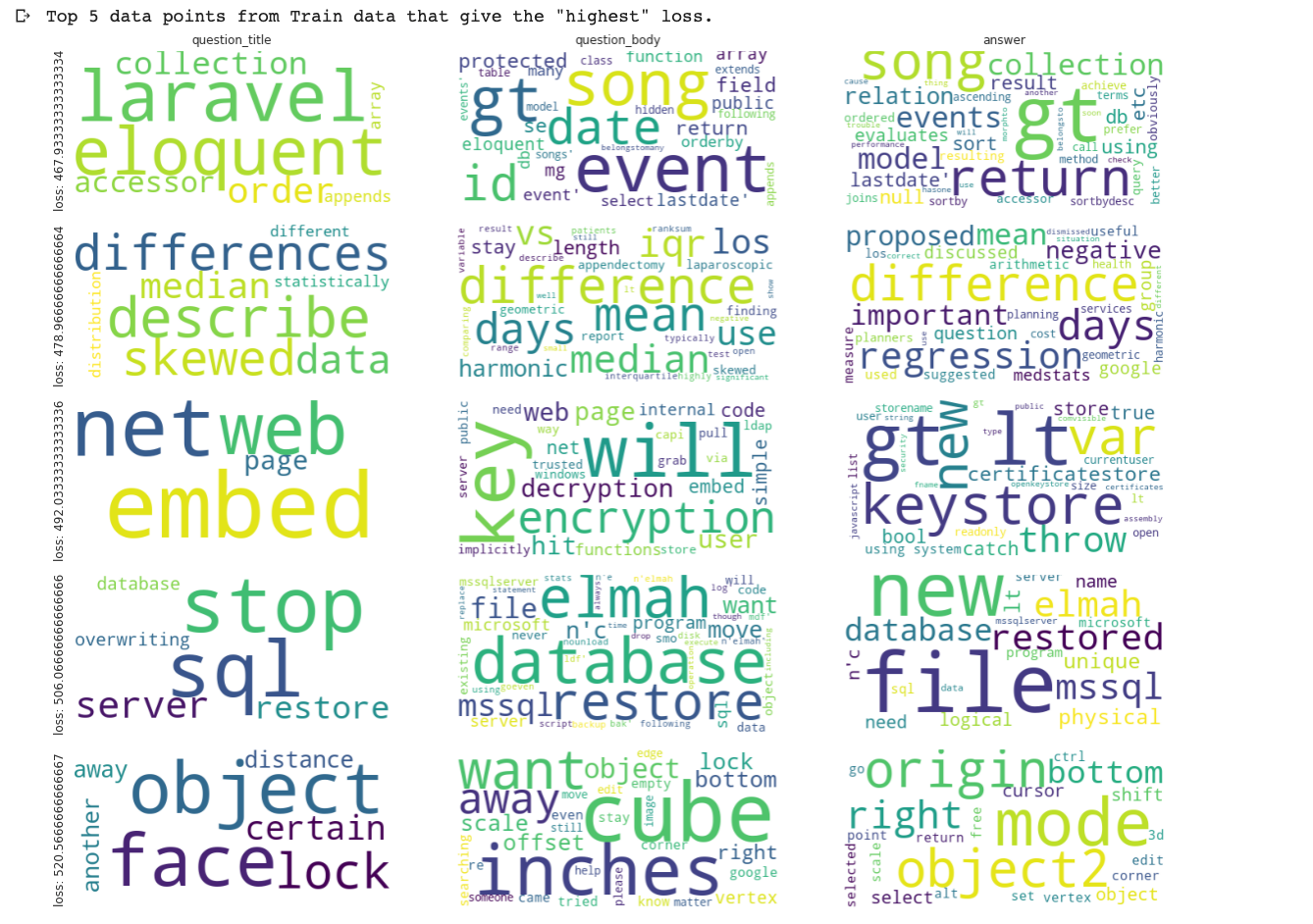
question_title, question_body, and answer
Starting with the first set of features, which are all text type features, I’ll be plotting word clouds using them. The plan is to segment out these features from 5 data-points that have the least scores and from another 5 data-points that have the most scores.
<iframe src="https://medium.com/media/67c8eb5b76d24a50287d02a4ff23efc6" frameborder=0></iframe>Let’s run the code and check what the results look like.
<iframe src="https://medium.com/media/87740269e9faed715110fe367f46e87d" frameborder=0></iframe>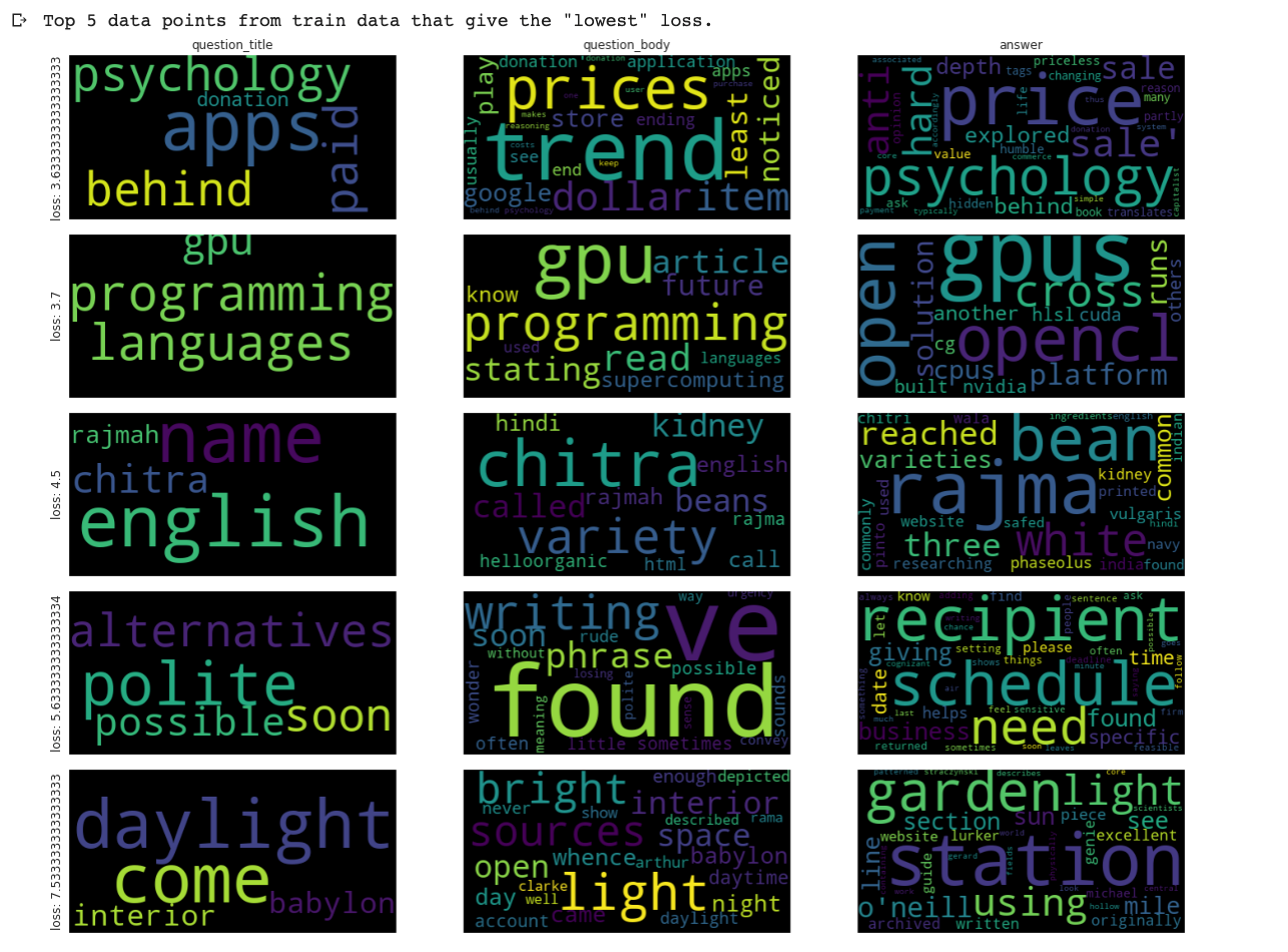
Word lengths of question_title, question_body, and answer
The next analysis is on the word lengths of question_title, question_body, and answer. For that, I’ll be picking 30 data-points that have the lowest MSE-scores and 30 data-points that have the highest MSE-scores for each of the 3 features question_title, question_body, and answer. Next, I’ll be calculating the word lengths of these 30 data-points for all the 3 features and plot them to see the trend.
<iframe src="https://medium.com/media/7f36671bb82d91c8f679916cf454ac70" frameborder=0></iframe>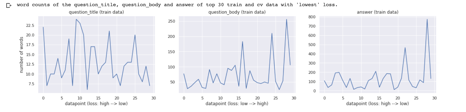

If we look at the number of words in question_title, question_body, and answer we can observe that the data that generates a high loss has a high number of words which means that the questions and answers are kind of thorough. So, the model does a good job when the questions and answers are concise.
host
The next analysis is on the feature host. For this feature, I’ll be picking 100 data-points that have the lowest MSE-scores and 100 data-points that have the highest MSE-scores and select the values in the feature host. Then I’ll be plotting a histogram of this categorical feature to see the distributions.
<iframe src="https://medium.com/media/7b314938018629724fbe3847921929aa" frameborder=0></iframe>

We can see that there are a lot of data points from the domain English, biology, sci-fi, physics that contribute to a lesser loss value whereas there are a lot of data points from drupal, programmers, tex that contribute to a higher loss.
Let’s also take a look at word-clouds of the unique host values that contribute to a low score and a high score. This analysis is again done using the top and bottom 100 data-points.
<iframe src="https://medium.com/media/874e00bdb6d24614915a30a94db933af" frameborder=0></iframe>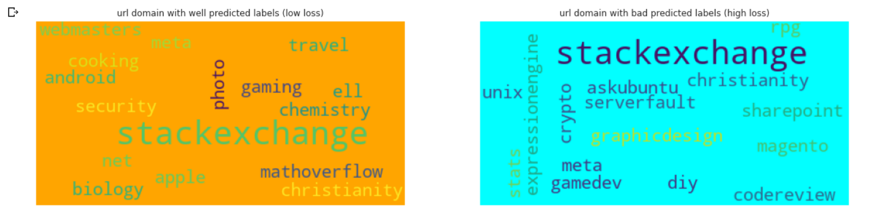
Category
The final analysis is on the feature category. For this feature, I’ll be picking 100 data-points that have the lowest MSE-scores and 100 data-points that have the highest MSE-scores and select the values in the feature category. Then I’ll be plotting a pie-chart of this categorical feature to see the proportions.
<iframe src="https://medium.com/media/86175a316237f88ea84e08d6966184ac" frameborder=0></iframe>
We can notice that datapoints with category as technology make up 50% of the data that the model could not predict well whereas categories like LIFE_ARTS, SCIENCE, and CULTURE contribute much less to bad predictions. For the good predictions, all the 5 categories contribute almost the same since there is no major difference in the proportion, still, we could say that the data-points with StackOverflow as the category contribute the least.
You can check the complete notebook on Kaggle using **this link** and leave an upvote if found my work useful.