The most challenging part of GRE preparation is the vocabulary part. At-least for me it was until my machine learning model helped me out with it.

When I started with my GRE preparation, after going through many resources (for the vocab section) I found that there are some words that pretty commonly appear in the exam and Barron’s high-frequency word list is one of the renowned resources that solve this problem. To begin with, I picked Barron’s 333 which is one such word list that contains 333 most frequently occurring words in GRE. The next challenge was learning these words so I came up with a plan. If I could somehow group similar words together it would make the learning process much easier. But how to do that? Manually grouping these words would be way more challenging than simply learning the words as they are. After pondering for some time, it occurred to me why not let the machine do all the hard work! I think with a capability of above one million million floating-point operations per second it is much better for these types of tasks than I am so let’s get started and see how to build a model from scratch that clusters similar words together.
I’ll be covering several machine learning concepts like Natural Language Processing (NLP), Term Frequency-Inverse Document Frequency (TF-IDF), Singular Value Decomposition (SVD), K-Means, t-Distributed Stochastic Neighbor Embedding (t-SNE) and many other techniques for data scraping, feature engineering and data visualization to demonstrate how we can cluster data from scratch.
Note: I’ll be using python 3.7 for this project.
The blog will be divided into the following parts-
-
Data collection: scraping websites to gather the data.
-
Data cleaning
-
Feature engineering
-
Modeling
-
Visualizing the results
Now that we know the problem statement and the data flow, let’s dive in.
Scraping the data
The first task is to collect the data i.e. Barron’s 333 high-frequency words. This can be done either by manually typing the words and creating a list or by automating the process. I used BeaulifulSoup and request to create a function that automatically scraped the data from different websites, let’s briefly understand the libraries and how to use them.
-
Numpy: A library adding support for large, multi-dimensional arrays and matrices, along with a large collection of high-level mathematical functions to operate on these arrays.
-
Pandas: A library written for data manipulation and analysis. In particular, it offers data structures and operations for manipulating numerical tables.
-
BeautifulSoup: A library for parsing HTML and XML documents. It creates a parse tree for parsed pages that can be used to extract data from HTML, which is useful for web scraping.
-
Requests: The requests module allows you to send HTTP requests using Python. The HTTP request returns a response object with all the response data (content, encoding, status, etc).
The code will use requests to get the response from the target websites, then using BeautifulSoup it’ll parse the html response and scrape out the required information from the page(s) and store the information in a tabular format using pandas. To understand the format of an html page, you can check out this tutorial.
# importing necessary libraries

import requests
from bs4 import BeautifulSoup
import re
from functools import reduce
import numpy as np
import pandas as pd
Let’s scrape the Barron’s 333 words and their meanings from this website-
{% highlight python linenos %} URL = "https://quizlet.com/2832581/barrons-333-high-frequency-words-flash-cards/" # url of the data we want to scrape. r = requests.get(URL) # request object collects server's response to the http request. soup = BeautifulSoup(r.content, 'html5lib') # BeautifulSoup creates a parser tree out of the html response that was collected using request. rows = soup.find_all('div', class_='SetPageTerm-inner') # Looking for elements with tag='div' and class_='SetPageTerm-inner'. dic = {} for row in rows: # iterating over all the elements. part = row.find_all('span', class_='TermText notranslate lang-en') # Looking for elements with tag='span' and class_='TermText notranslate lang-en' word = part[0].text # collecting the words. meaning = part[1].text # collecting the meaning. dic[word] = meaning # adding the word, meaning to dictionary as key value pairs. df = pd.DataFrame(dic.items(), columns=['word', 'meaning']) # converting to dataframe {% endhighlight %}
The HTML code of a webpage in chrome can be accessed using ⌘+shift+c on mac or ctrl+shift+c on windows/Linux.
Here I’m using ‘span’ as tag, class_= ‘TermText notranslate lang-en’ since the elements containing word and meaning have the same tag and class and there are only 2 such elements in every row element, 1st one corresponding to word and the 2nd one to the meaning.

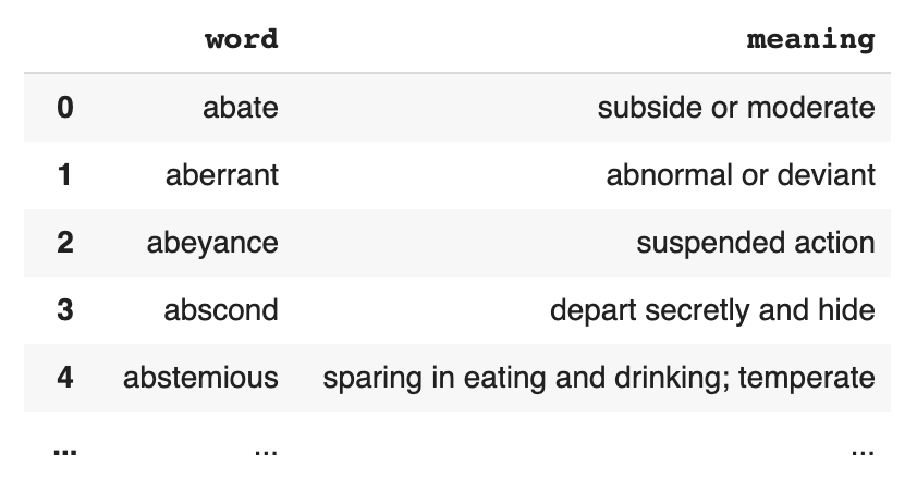
This is the scraped data in tabular form.
This data is not enough so let’s add more data by scraping the synonyms of each word from this website-
{% highlight python linenos %} def synonyms(word, th=20): URL = f"https://www.thesaurus.com/browse/{word}" # this url returns the page with 'word' described r = requests.get(URL) # collecting the http response from the url soup = BeautifulSoup(r.content, 'html5lib') # parsing the html page to extract items. rows = soup.find_all('span', class_ = 'css-133coio etbu2a32') # stores all the element containing synonyms of the word. syn = [word] if(len(rows)<th): # here, th denotes the number of synonyms that we need. th = len(rows) # in some cases only limited synonyms were available so I modified the code a bit. for r in rows[:th]: # iterating over all the elements containing synonyms try: syn.append(r.a.text) # scrapping synonym string and storing in a list (most of them have a tag='a') except: syn.append(r.span.text) # scrapping synonym string with tag='span' return syn
from tqdm import tqdm_notebook mapping = [] # stores the word and it's synonyms for word in tqdm_notebook(df.word.values): # iterating over the words and scrapping synonyms syn = synonyms(word, th=3) # I'll be collecting 5 synonyms mapping.append(syn) # storing the synonyms.
data = pd.DataFrame(mapping) # Converting to dataframe data.columns = ['word','synonym_1','synonym_2','synonym_3','synonym_4','synonym_5'] {% endhighlight %}


Now let’s join the 2 data frames (meanings and synonyms):
result = pd.merge(df.word, data, on='word')
result.fillna('', inplace=True)
print(result)

We can see the data needs some cleaning since it contains stop-words like and, or, the and other elements like punctuation marks. Also, we must take care of the contractions like can’t, won’t, don’t these must be converted to can not, would not, do not respectively.
{% highlight python linenos %} from nltk.corpus import stopwords def preprocess(sentence): stop_words = ['ourselves', 'hers', 'between', 'yourself', 'but', 'again', 'there', 'about', 'once', 'during', 'out', 'very', 'having', 'with', 'they', 'own', 'an', 'be', 'some', 'for', 'do', 'its', 'yours', 'such', 'into', 'of', 'most', 'itself', 'other', 'off', 'is', 's', 'am', 'or', 'who', 'as', 'from', 'him', 'each', 'the', 'themselves', 'until', 'below', 'are', 'we', 'these', 'your', 'his', 'through', 'don', 'nor', 'me', 'were', 'her', 'more', 'himself', 'this', 'down', 'should', 'our', 'their', 'while', 'above', 'both', 'up', 'to', 'ours', 'had', 'she', 'all', 'no', 'when', 'at', 'any', 'before', 'them', 'same', 'and', 'been', 'have', 'in', 'will', 'on', 'does', 'yourselves', 'then', 'that', 'because', 'what', 'over', 'why', 'so', 'can', 'did', 'not', 'now', 'under', 'he', 'you', 'herself', 'has', 'just', 'where', 'too', 'only', 'myself', 'which', 'those', 'i', 'after', 'few', 'whom', 't', 'being', 'if', 'theirs', 'my', 'against', 'a', 'by', 'doing', 'it', 'how', 'further', 'was', 'here', 'than'] sentence_clean = [words if words not in stop_words else '' for words in sentence.split(' ')] sentence = ' '.join(sentence_clean) sentence = re.sub(';', '', sentence) sentence = re.sub('(', '', sentence) sentence = re.sub(')', '', sentence) sentence = re.sub(',', '', sentence) sentence = re.sub('-', ' ', sentence) sentence = re.sub('\d', '', sentence) sentence = re.sub(' ', ' ', sentence) sentence = re.sub(r"won't", "will not", sentence) sentence = re.sub(r"can't", "can not", sentence) sentence = re.sub(r"n't", " not", sentence) sentence = re.sub(r"'re", " are", sentence) sentence = re.sub(r"'s", " is", sentence) sentence = re.sub(r"'d", " would", sentence) sentence = re.sub(r"'ll", " will", sentence) sentence = re.sub(r"'t", " not", sentence) sentence = re.sub(r"'ve", " have", sentence) sentence = re.sub(r"'m", " am", sentence) return sentence {% endhighlight %}
Now since the data has been cleaned, let’s do some feature engineering.
Feature engineering
One thing that I noticed was that some of these words have synonyms that also belong to Barron’s 333 list. If I could somehow concatenate the synonyms of these words, it could increase the performance of our model.

-
Eg. for Tortuous, the synonyms are circuitous, convoluted, indirect.
-
Out of the 3 synonyms, convoluted is present in Barron’s 333-word list and its synonyms are intricate, labyrinthine, perplexing.
-
So, the final synonyms of tortuous should be circuitous, convoluted, indirect, intricate, labyrinthine, perplexing.
After this step, for each word in Barron’s 333-word list we have, it’s direct synonyms, indirect synonyms (in the above example, the synonyms of convoluted are the indirect synonyms of tortuous) and meaning. I’ll use the notation set for this data further in this blog.
Set: data about a word (here the word is from barron’s 333) like it’s direct synonyms, indirect synonyms and meaning. The set of a word includes the word itself.
We have obtained clean sets of words that we need to cluster but remember we first need to convert these sets into some kind of numerical data because our model needs numbers to work on.
I’ll use TF-IDF to vectorize the data. Before diving in let’s understand what tf-idf is-
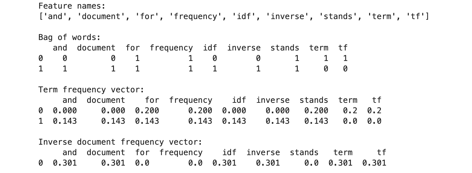
TF-IDF short for term frequency-inverse document frequency is a numerical statistic that is intended to reflect how important a word is to a document in a corpus. Let’s understand this using Bag of Words.
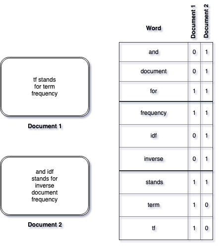
The bag-of-words model is a simplifying representation used in natural language processing and information retrieval. In this model, a text is represented as the bag of its words. In simple terms, Bag of Words is nothing but a basic numerical representation of documents, it is done by first creating a vocabulary of words that contains all the distinct words from all the documents. Now each document is represented using a vector that has ‘n’ elements (here, n is the number of words in the vocabulary so each element corresponds to a word in the vocabulary) and each element has a numerical value that tells us how many times that word was seen in that document. let’s consider an example:
-
The column word represents the vocabulary.
-
In the table, column Document 1 and Document 2 represent the BOW of documents 1 and 2 respectively.
-
The numbers represent how many times the corresponding word occurs in the document.
-
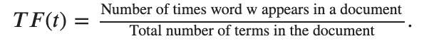
Now comes TF-IDF, it is simply the product of term frequency and inverse document frequency.
Term frequency: It is the number that represents how often a word is present in the document.
Inverse document frequency: It is the inverse of the log of the chance of finding a document that has the word in it.
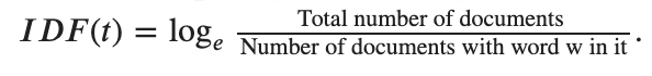
Think about it this way: If the word is used extensively in all documents, its existence within a specific document will not be able to provide as much specific information about the document itself. So the second term could be seen as a penalty term that penalizes common words such as “a”, “the”, “and”, etc. tf-idf can, therefore, be seen as a weighting scheme for words relevancy in a specific document.
Let’s check the TF-IDF of the two documents: Document 1: “tf stands for term frequency”, terms: 5 Document 2: “and idf stands for inverse document frequency”, terms: 7

Bi-grams: A bigram is a sequence of two adjacent elements from a string of tokens, which are typical letters, syllables, or words. Here is an example of uni-grams and bi-grams generated from a document.
doc: “tf stands for term frequency”
uni-grams: [‘tf’, ‘stands’, ‘for’, ‘term’, ‘frequency’]
bi-grams: [‘tf stands’, ‘stands for’, ‘for term’, ‘term frequency’]
The advantage of n-grams is that they add information about the sequence of words in a document.
I’ve written a function for calculating the TF-IDF, the function uses both uni-grams and bi-grams.
{% highlight python linenos %} class tfidf_vectorizer: def init(self): self.n_grams = [] self.tf = [] self.idf = [] self.vocab = [] self.tfidf_ = []
def fit(self, data):
  '''This function generates the vocabulary.
  Here I've used both uni-grams and bi-grams.'''
    uni_grams = set()
    bi_grams = set()
    for rows in data:
        words = rows.split(' ')
        for word_pair in zip(words, words[1:]):
            uni_grams.add(word_pair[0])
            bi_grams.add(word_pair)
        uni_grams.add(word_pair[1])
    self.n_grams = list(uni_grams.union(bi_grams))

def transform(self, data):
  '''This function calculates the tf values for each document, idf values for each word
  and then finally returns the tfidf values'''
    tf_ = pd.DataFrame(columns=[self.n_grams])
    idf_ = dict.fromkeys(self.n_grams, 0)
    idf_list = [1]*len(self.n_grams)
    for idx,rows in enumerate(data):
        words = rows.split(' ')
        tf = dict.fromkeys(self.n_grams, 0)
        for word_pair in zip(words, words[1:]):
            tf[word_pair] += 1
            tf[word_pair[0]] += 1
            idf_[word_pair] = 1
            idf_[word_pair[0]] += 1
        tf[word_pair[1]] += 1
        idf_[word_pair[1]] += 1
        idf_list += np.array(list(idf_.values()))
        vector = np.array(list(tf.values()))
        vector = vector/len(words)
        tf_.loc[idx] = vector
    # print(idf_list)
    idf_ = np.array([np.log(len(data)/term) for term in idf_list])
    idf_ = nz.fit_transform(idf_.reshape(1, -1))[0]
    tfidf_ = tf_.values*idf_
    self.tf = tf_
    self.idf = idf_
    return tfidf_

def fit_transform(self, data):
  '''This function performs both fit and transform'''
    fit_ = fit(self, data)
    transform_ = transform(self, data)
    return transform_
{% endhighlight %}
Now, that we have the TF-IDF embeddings for each of the sets, we can proceed to modeling.
Note: The data we have till now is in a tabular form containing m rows and n columns where ‘m’ is the number of words in Barron’s 333-word list and ‘n’ is the size of Bag of Words vocabulary. This tabular data can also be represented as an array of dimension (m x n). Further in the blog, I’ll be using array to represent the data.
Before Modeling there is something that I would like to share that I found very helpful. Instead of using the TF-IDF values directly for modeling, how about bringing down the dimensions of the data? That means, we have TF-IDF values corresponding to each set and since these TF-IDF values are represented as a vector of n elements, where ‘n’ also corresponds to the number of distinct words in all of our sets. If 2 sets have almost the same words, the distance between there corresponding points in an n-dimensional hyperplane is going to be very less and vice-versa. Similarly, if the 2 sets have very less words in common, the distance between there corresponding points in n-hyperplane is going to be much more and vice-versa. Now instead of using n-hyperplane to represent these points, I reduced the dimensionality of the points to 32-dimensions (Why 32? is discussed later in the blog). The dimensionality can be reduced by picking 32 random dimensions and ignoring the others but that would just be too stupid, so I tried using different dimensionality reduction techniques and found Truncated SVD to work miracles for the given data.
I used dimensionality reduction as a method to add some form of regularization to the data.
Let’s understand Truncated SVD-
SVD abbreviation for Singular Value Decomposition is a matrix factorization technique that factorizes any given matrix into the three matrices U, S, and V. It goes by the equation-

Let me explain what U, S, and V are.
U (aka left singular): is an orthogonal matrix whose columns are the eigenvectors of AᵀA.
S (singular): is a diagonal matrix whose diagonal elements are the square root of eigenvalues of AᵀA or AAᵀ(both have the same Eigenvalues) arranged in descending order i.e.

V (aka right singular): is an orthogonal matrix whose columns are the eigenvectors of AAᵀ*.*

Eigenvectors: An eigenvector is a vector whose direction remains unchanged when a linear transformation is applied to it. Consider the image below in which three vectors are shown. The green square is only drawn to illustrate the linear transformation that is applied to each of these three vectors.
Note that the direction of these eigenvectors do not change but their length does change, and eigenvalue is the factor by which their length change.
source: https://www.visiondummy.com/2014/03/eigenvalues-eigenvectors/

So now that we know how to factorize a matrix, we can reduce the dimension of a matrix using Truncated SVD which is a simple extension to SVD.
Truncated SVD: Suppose we have an input matrix of dimensions (m x n) which we want to reduce to (m x r) where r<n. We simply compute the first ‘r’ eigenvectors of AᵀA and store it as the columns of U, then we compute the first ‘r’ eigenvectors of AAᵀ and store it as the columns of V and finally the root of first ‘r’ eigenvalues as diagonal elements of S.
So in a nutshell, Truncated-SVD is a smart technique that reduces the dimensionality of given data in a smart way by preserving as much information (variance) as possible.
If you want to dive deeper into SVD, check out this lecture by Prof. W. Gilbert Strang, and this wonderful blog on SVD.
Scikit-learn comes with Truncated SVD built in that can be imported and used directly.
Modeling
Now that we are done with the data pre-processing and feature engineering part, let’s see how to group similar words together using a clustering algorithm.
K-means clustering is a type of unsupervised learning, which is used when you have unlabeled data (i.e., data without defined categories or groups). The goal of this algorithm is to find groups in the data, with the number of groups represented by the variable K.
Let’s see how K-means works. Suppose there are some points in a 2-dimensional plane, and we want to cluster these points into K clusters.

The steps are simple-
-
Defining K points randomly in the plane. Let’s call these points as cluster centroids.
-
Iterating over each point in the data and check for the closest centroid and assign that point to its closest centroid.
-
After the above step, each centroid must have some points that are closest to it, let’s call these sets of points clusters.
-
Updating the centroid of each cluster by calculating the mean value of x and y coordinate of all the points in that cluster. The calculated mean values (x, y) are the coordinates of the updated centroid of that cluster.
-
Repeating the last 3 steps until the coordinates of the centroids do not update much.
But how to decide the right value for K (number of clusters)? Let’s define a metric that can be used to measure the right value of K. Distortion is one such metric that uses the sum of squares of the distance of points in a cluster from the cluster mean, for all the clusters summed up.

Distortion can be used to check how efficient the clustering algorithm is for a given value of K.
The optimal value of K can be determined by calculating the distortion value for different values of K and then plotting them.
This plot is known as the Elbow plot. Just by looking at the elbow plot we can determine the optimal ‘K’ as the value where distortion stops decreasing rapidly.
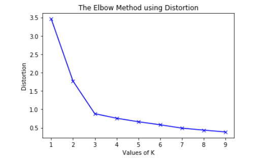
Here is an Elbow plot and just by looking at it, we can say that the best hyperparameter is k=3.
It is called elbow plot because it looks like an arm (maybe a stick man’s arm) and the elbow of this arm represents the optimal K.
One more thing, I’ll be using cosine distance as a measure to compute the distance between points (including centroids). Let’s quickly understand what cosine distance is using cosine similarity.

Cosine similarity is a measure to calculate how parallel 2 vectors are. It is calculated using the cosine of the angle between 2 vectors. It can easily be calculated using-

So if 2 vectors a and b are parallel, the angle between them will be 0 and the cosine similarity will be cos(0) = 1. Similarly, if 2 vectors a and b are pointing in the opposite direction, the angle between them will be 𝛑 and the cosine similarity will be cos(𝛑) = -1.
In a nutshell, cosine similarity tells us about what extent 2 vectors are pointing in a similar direction. A value near 1 tells us that the vectors are pointing in a very similar direction whereas a value near -1 corresponds to pointing in opposite directions.

Now Cosine distance between 2 points is nothing but
1 - (cosine similarity of the vectors representing them in hyperspace).
So it ranges from (0 to 2), where 0 corresponds to the points being very similar, and 2 corresponds to the points being very dissimilar.
Can you guess when will the cosine distance between 2 points be 1?
To know more check out this blog.
I’ll be implementing K-means from scratch since Scikit learns K-Means does not support cosine distance.
{% highlight python linenos %} class KMeans: def init(self, n_clusters): self.n_clusters = n_clusters # initializing the number of clusters
def fit(self, df): # This function performs fit operation on the data
    df = pd.DataFrame(df)
    self.data = df.copy()
    self.clusters = np.zeros(self.data.shape[0]) # initializing the clusters as all zeros

    # initializing centroids
    rows = self.data
    rows.reset_index(drop=True, inplace=True)
    self.centroids = rows.sample(n=self.n_clusters)
    self.centroids.reset_index(drop=True, inplace=True)

    # Initialize old centroids as all zeros
    self.old_centroids = pd.DataFrame(np.zeros(shape=(self.n_clusters, self.data.shape[1])),
                                      columns=self.data.columns)

    # check the distance of each data point to the centroid and assigning each point to the closest cluster.
    while not self.old_centroids.equals(self.centroids):
        # Stash old centroids
        self.old_centroids = self.centroids.copy(deep=True)

        # Iterate through each data point/set
        for row_i in range(0, len(self.data)):
            distances = list()
            point = self.data.iloc[row_i]

            # Calculate the distance between the point and centroid
            for row_c in range(0, len(self.centroids)):
                centroid = self.centroids.iloc[row_c]
                point_array = np.array(point).reshape(1,-1)
                centroid_array = np.array(centroid).reshape(1,-1)
                distances.append(cosine_distances(point_array, centroid_array)[0][0])

            # Assign this data point to a cluster
            self.clusters[row_i] = int(np.argmin(distances))

        # For each cluster extract the values which now belong to each cluster and calculate new k-means
        for label in range(0, self.n_clusters):

            label_idx = np.where(self.clusters == label)[0]

            if len(label_idx) == 0:
                self.centroids.loc[label] = self.old_centroids.loc[label]
            else:
                # Set the new centroid to the mean value of the data points within this cluster
                self.centroids.loc[label] = self.data.iloc[label_idx].mean()
{% endhighlight %}
It’s time to run the algorithm on the pre-processed data and check for the right hyperparameters. Hyperparameter tuning is a process of determining the right hyperparameters that make the model work phenomenally well for the given data. In this case, there are 2 hyperparameters-
-
1 from Truncated-SVD: n_components (reduced dimension)
-
1 from K-means: ‘K’ (number of clusters).
I’ve already plotted the elbow plots for different n_component values.
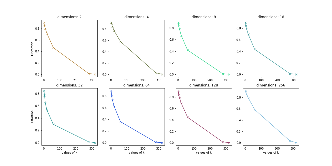
By looking at the plots, we can say that the best hyperparameters are-
- n_components: 32
- K (number of clusters): 50
Finally, It’s time to initialize Truncated-SVD and K-Means using the best hyperparameters and cluster the data.
from sklearn.decomposition import TruncatedSVD

> trans = TruncatedSVD(n_components=32)
> data_updated = trans.fit_transform(words_tfidf.toarray())
> model = custom_KMeans(n_clusters=50)
> model.train(data_updated)
Visualizing the results
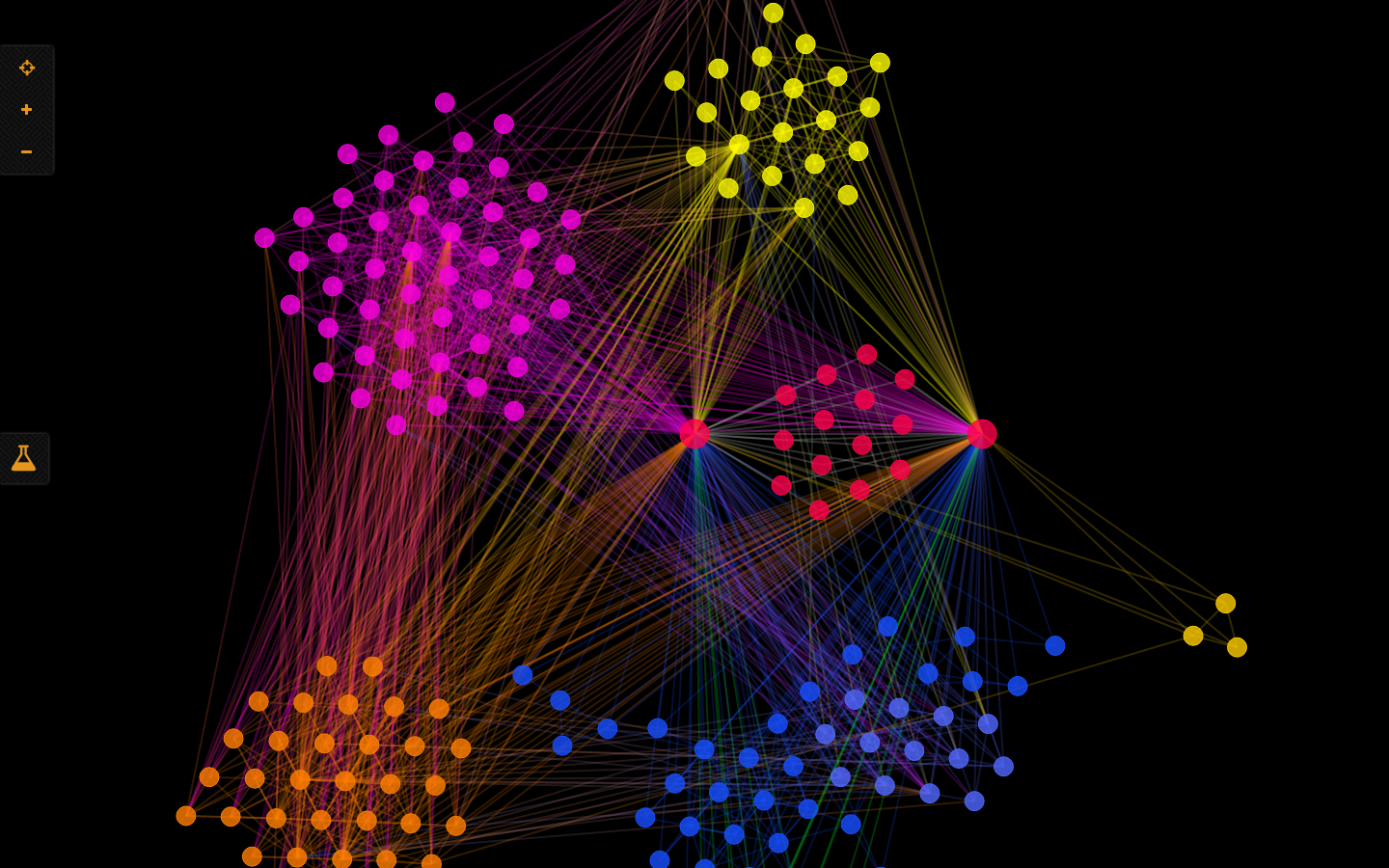
These are the results obtained after clustering the data.

Let’s check out some of the clusters:
I’ll be using the networkx library to create the clusters.
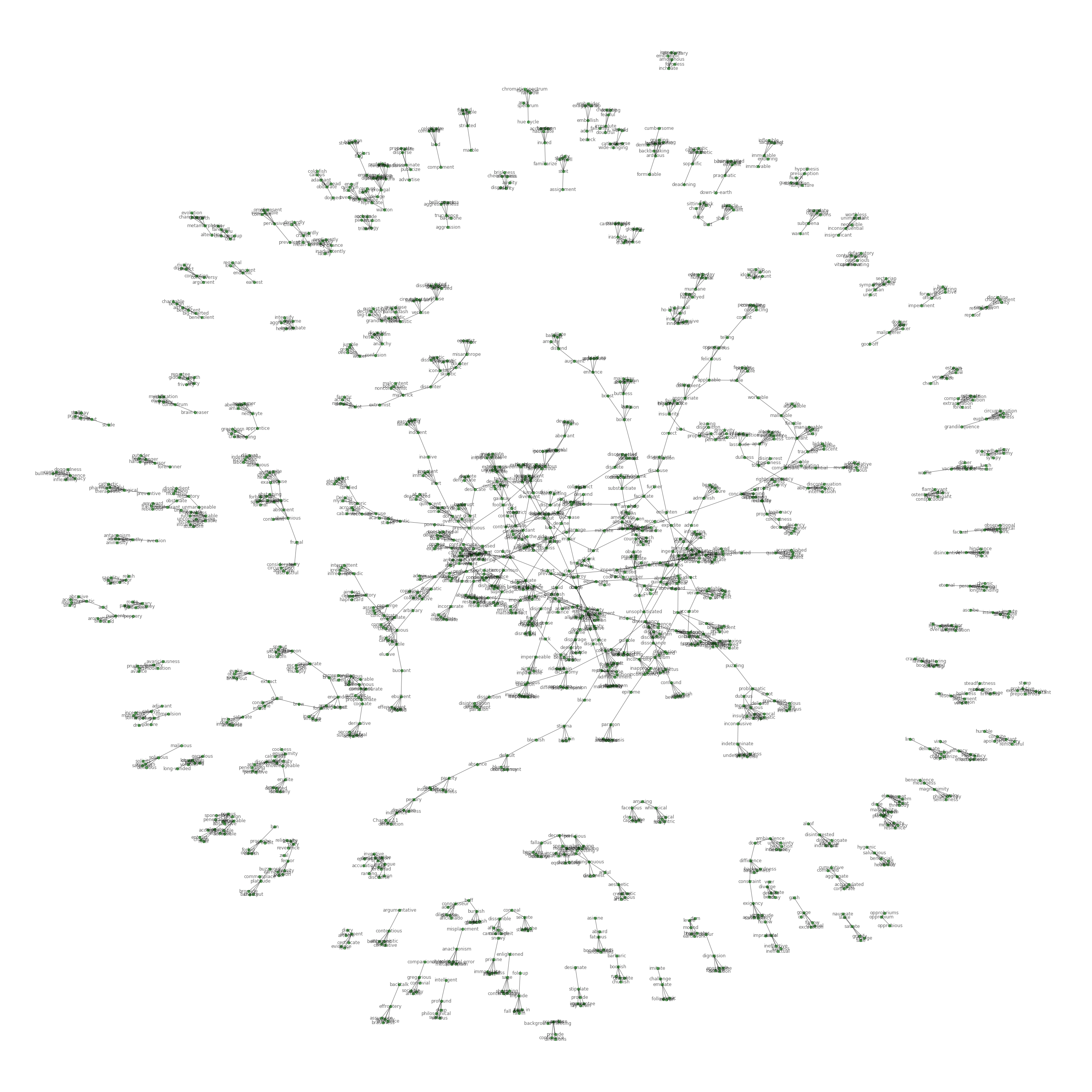
In each cluster, the red nodes correspond to the words from Barron's 333-word list and how they are linked with each other and their synonyms.
You can check out the documentation for networkx here. Also, I’ll demonstrate how wonderful it is with an example in the end.

Finally, let’s visualize the data in 3d using t-SNE but first,
Let’s talk about t-SNE:

t-SNE (t-Distributed Stochastic Neighbor Embedding) is a non-linear dimensionality reduction algorithm used for exploring high-dimensional data. It maps multi-dimensional data to two or more dimensions such that each embedding in the lower dimension represents the value in higher dimension. Also, these embeddings are placed in the lower dimension in such a manner that the distance between neighborhood points is preserved. So, t-SNE preserves the local structure of the data as well.
I’ll try to explain how it does what it does.
For a given point in n-dimensional hyperspace, it calculates the distance of that point from all the other points and converts these distributions of distances to student’s t-distribution. This is done for all the points such that in the end, each point has its own t-distribution of distances from all the other points.
Now the points are randomly scattered in the lower dimensional space and each point is displaced by some distance such that after the displacement of all the points is done if we recalculate the t-distribution of distances of each point from the remaining points (this time this is done in the lower dimensional space), the distribution would be the same as what we obtained in n-dimensional hyperspace.
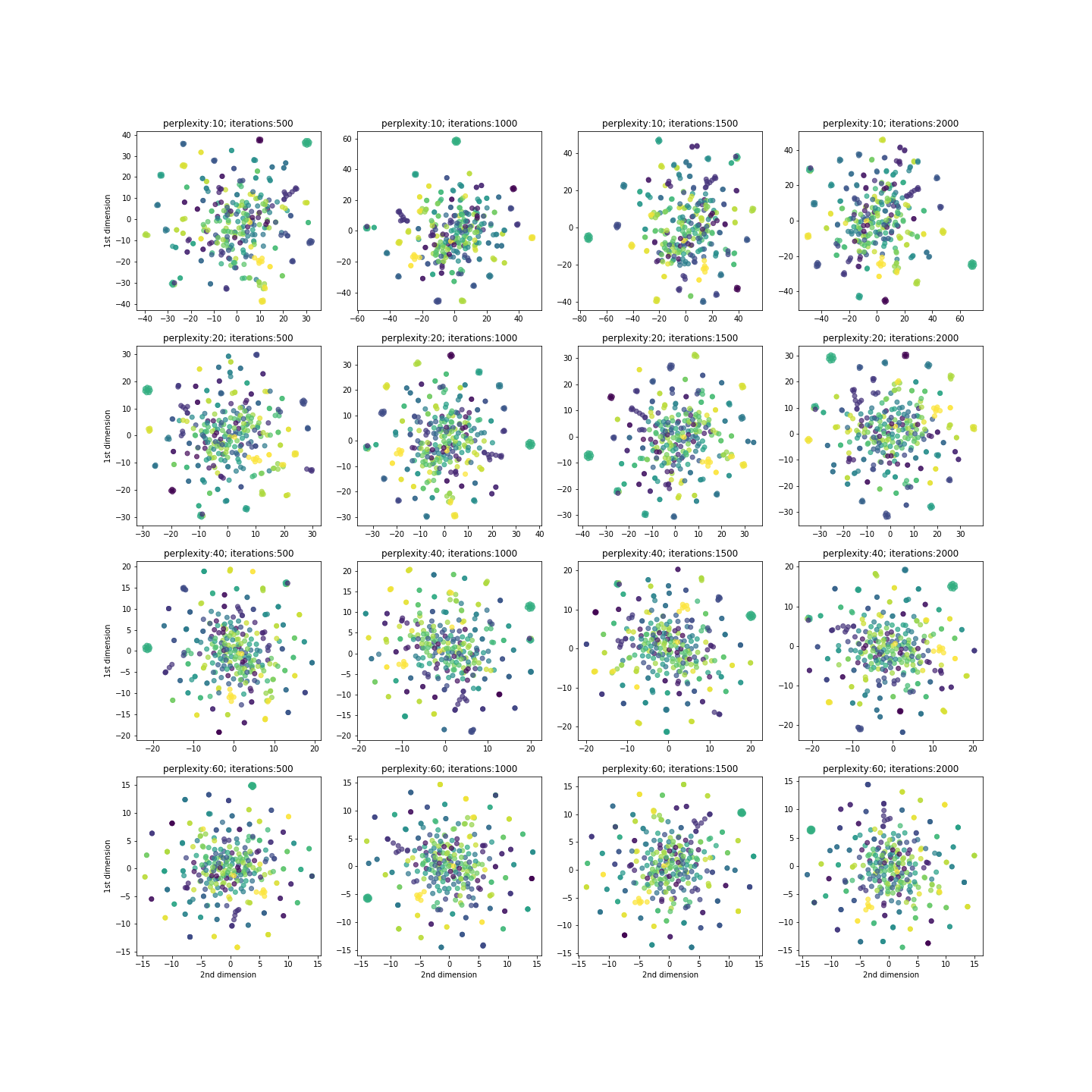
There are 2 main hyperparameters in t-SNE-
Perplexity: Instead of calculating the distance from all the other points, we can use only ‘k’ nearest points. This value of ‘k’ is called the perplexity value.
Iterations: The number of iterations for which we want t-SNE to update the points in lower-dimensional space.
Due to stochasticity, the algorithm may perform differently for different perplexity values so as a good practice, it is preferred to run t-SNE for different perplexity values and different numbers of iterations.
To know more about t-SNE, check out this awesome blog, it has t-SNE very well explained with interactive visualization.
Below is the plot using t-SNE in two dimensions for different perplexity and iteration values. We can see t-SNE working well with perplexity 20 and 2000 iterations.
{% highlight python linenos %}
from sklearn.manifold import TSNE import matplotlib.pyplot as plt from tqdm import tqdm_notebook
f, ax = plt.subplots(4,4, figsize=(20,20))
trans = TruncatedSVD(n_components=32) svd_dim = trans.fit_transform(words_tfidf.toarray())
perplexity = [10,20,40,60] iterations = [500,1000,1500,2000] p_= 0 for p in tqdm_notebook(perplexity): i_ = 0 for i in tqdm_notebook(iterations): trans_ = TSNE(n_components=2, perplexity=p, n_iter=i) node_embeddings_2d = trans_.fit_transform(svd_dim) ax[p_,i_].scatter(node_embeddings_2d[:,0], node_embeddings_2d[:,1], c=clf.clusters, alpha=0.7) ax[p_, i_].set_title(f'perplexity:{p}; iterations:{i}') if i_==0: ax[p_, i_].set_ylabel('1st dimension') if p_==3: ax[p_, i_].set_xlabel('2nd dimension') i_+=1 p_+=1 plt.savefig('tsne_plot.png') plt.show() {% endhighlight %}
Finally, Here is the complete graph of all the words and their synonyms (I used 4 synonyms for each word) using networkx.
{% highlight python linenos %}
import networkx as nx from networkx.algorithms import bipartite import matplotlib.pyplot as plt
data = pd.read_csv('barrons333_4.csv') # contains word-synonym pair
edges = [tuple(x) for x in data.values.tolist()]
B = nx.Graph() B.add_nodes_from(data['word'].unique(), bipartite=0, label='word') B.add_edges_from(edges, label='links')
pos_ = nx.spring_layout(B)
plt.figure(figsize=(45,45)) nx.draw(B, with_labels=True, pos=pos_, node_color='gray', edge_color='gray', node_size=50, alpha=0.6) word_list = list(data['word'].unique()) nx.draw_networkx_nodes(B, pos=pos_, nodelist=word_list, ... node_size=100, node_color='g', alpha=0.6) plt.show() {% endhighlight %}
Final note
Thank you for reading the blog. I hope it was useful for some of you aspiring to do projects on NLP, unsupervised machine-learning, data processing, data visualizing.
And if you have any doubts regarding this project, please leave a comment in the response section or in the GitHub repo of this project.
The full project is available on my Github: https://github.com/SarthakV7/Clustering-Barron-s-333-word-list-using-unsupervised-machine-learning
Find me on LinkedIn: www.linkedin.com/in/sarthak-vajpayee
Peace! ☮