Nature paper

This repo is related to our paper that came out in Nature. Please cite it as:

Greene, C.A., Gardner, A.S., Wood, M. et al. Ubiquitous acceleration in Greenland Ice Sheet calving from 1985 to 2022. Nature 625, 523–528 (2024). https://doi.org/10.1038/s41586-023-06863-2

Greenland monthly ice masks

MATLAB scripts to combine terminus picks into a consistent gridded ice mask.

Data access

The final data product is a gridded, time-evolving Greenland ice mask at 120 m spatial resolution, posted at monthly intervals from 1972 to 2022 (use caution before 1985 due to data limitations). The ice masks are presented in NetCDF format, along with ice velocity and thickness data here: https://www.doi.org/10.5067/579TO87M7IZB

Citation

If you use this data, please cite our paper!

Greene, C.A., Gardner, A.S., Wood, M. et al. Ubiquitous acceleration in Greenland Ice Sheet calving from 1985 to 2022. Nature. https://doi.org/10.1038/s41586-023-06863-2

animations folder contains a few gifs. Hundreds more animations are made for quality-control checks by greenland_icemask_animations_for_qc.m, but those animations are stored with the data because of filesize limitations.
code folder contains all code necessary to create monthly ice masks, analyze the data, and create the figures published in our manuscript.
data folder contains final and intermediate data products.
figures folder contains all of the figures in our manuscript, plus a few figures that didn't make it into the manuscript.

Workflow

thickness_inversion_uncertainty.m explores the uncertainty associated with inverting bed elevations to solve for approximate thickness in fjords where ice no longer exists. In the map below, the edge of a semi-transparent blue ice sheet cuts diagonally across the image. Orange grid cells indicate locations where the BedMachine ice sheet edge is grounded below sea level and errbed is less than 100 m. For all such pixels around the ice sheet perimeter, we find that the BedMachine thickness is, on average, about 5% greater than H_eq, the minimum thickness necessary for the ice to be grounded. When we invert BedMachine bed elevations to obtain hydrostatic-equilibrium thickness and multiply by 1.05, our inverted thickness matches BedMachine thickness within ±32.7 m.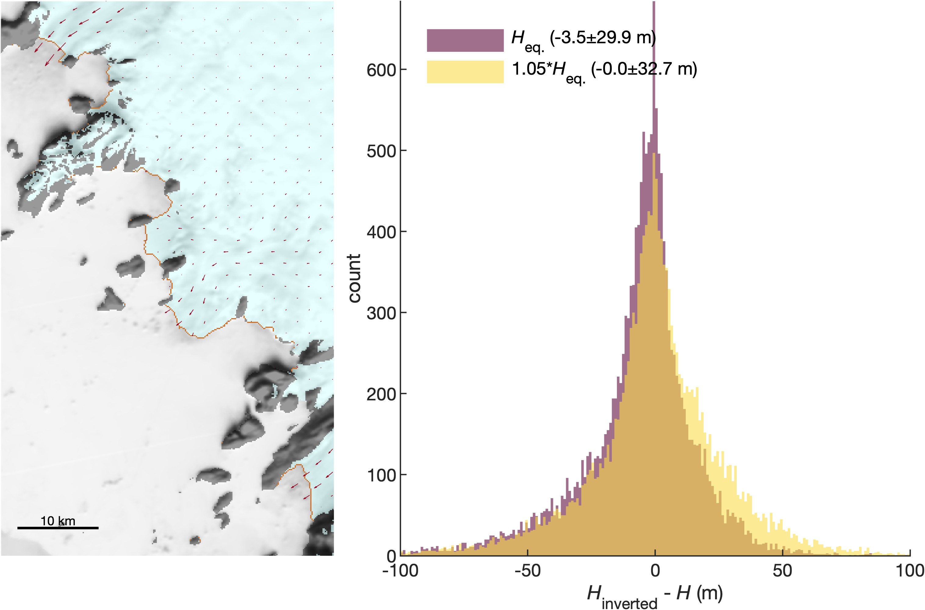
AERODEM_cleaner.m removes questionable data from AERODEM and creates aerodem_clean.mat.
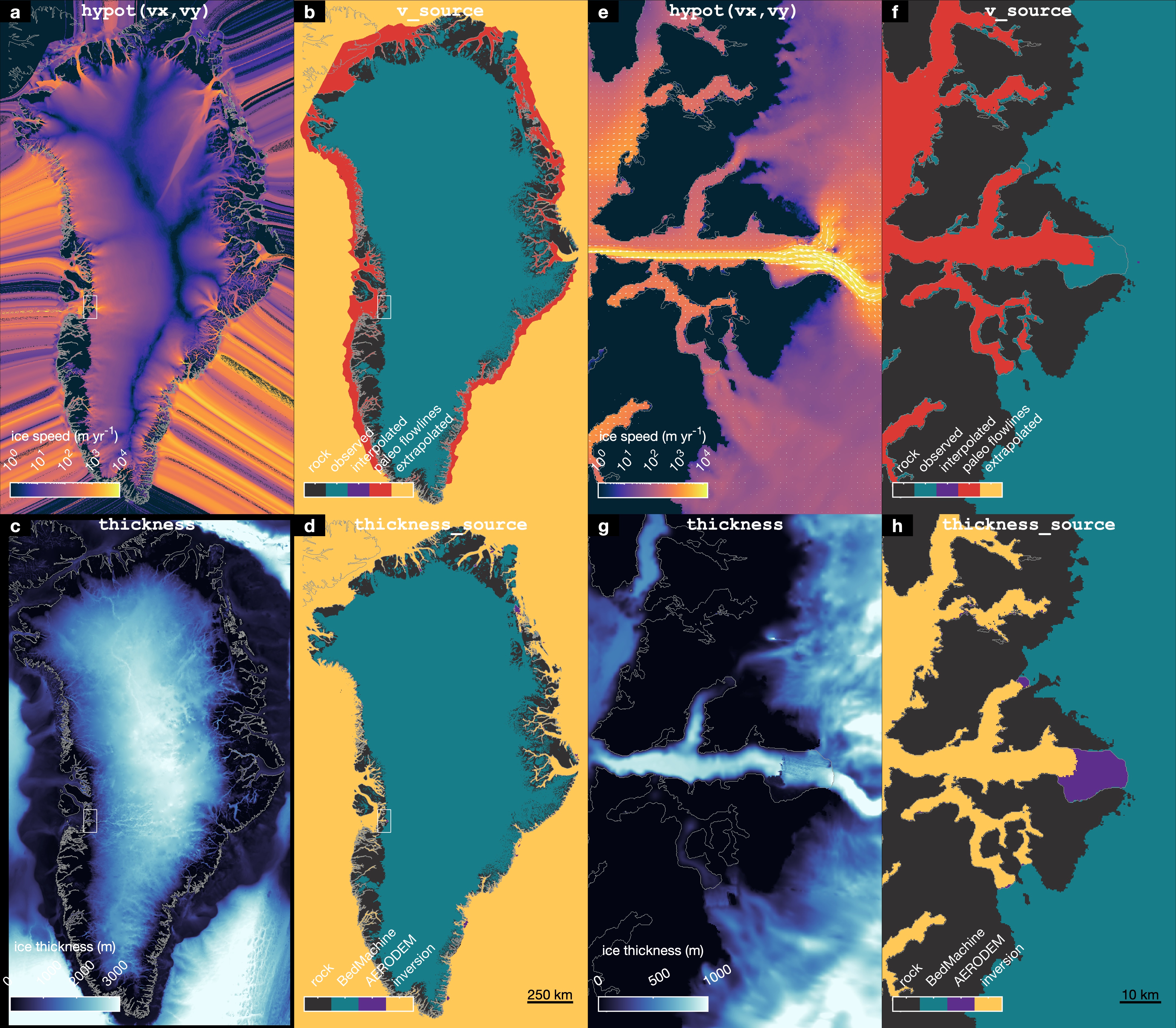
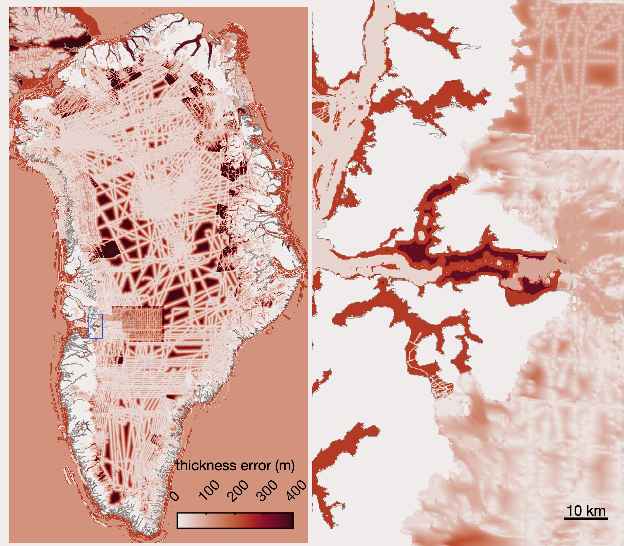
greenland_extrude_velocity_and_thickness_v2.m takes ITS_LIVE v2 velocities, fills in missing data with paleo modeled velocities wherever possible, and then extrapolates beyond all measured and modeled extents to fill the entire domain. This script also extrapolates BedMachine v5 thickness in the direction of the extrapolated velocities.
- This script creates greenland_extruded_velocity_and_thickness_2022-12-15.nc.
- Requirements:
- Run greenland_extruded_velocity_and_thickness_plotter.m afterward to view the extruded velocity and thickness data, and make these:
measures_terminuspicks_compiler.m compiles all annual shapefile data from Joughin et al., 2021 into a single .mat file. Put all 49 years of shapefile data into a single folder then run this script.
- This script creates measures_greenland_terminus_picks_v2.mat.
- Requirements:
  - MATLAB's Mapping Toolbox (for shaperead) and
  - MEaSUREs Annual Greenland Outlet Glacier Terminus Positions from SAR Mosaics, Version 2 shapefile data.
autoterm_data_reformatter.m combines shapefile data from AutoTerm into a single .mat file, in a shapefile-like structure that's easy to combine with shapefiles from the other datasets. This script only saves data that meet certain error quality thresholds, which have already been defined on a per-glacier basis by manual inspection and can be found in autoterm_error_thresholds.mat. This script saves autoterm_reformatted_trimmed.mat.
terminus_data_densifier.m reads in terminus position shapefiles from TermPicks (Goliber et al.), CALFIN (Cheng et al.), MEaSUREs v2 (Joughin et al.), and AutoTerm (Zhang et al.).
- This script:
  
  a. Compiles terminus position data from TermPicks (Goliber et al.), CALFIN (Cheng et al.), MEaSUREs v2 (Joughin et al.), and AutoTerm (Zhang et al.). There is no terminus data in 1983. Here is the distribution of all the 63,473 terminus position picks:
  b. Densifies terminus position shapefiles to make about 5 points per grid cell width. Here's an example, which shows 263 datapoints in a two-segment piece of a TermPicks terminus position of Jakobshavn from March 3, 2005. The red dots are densified to 24 m spacing.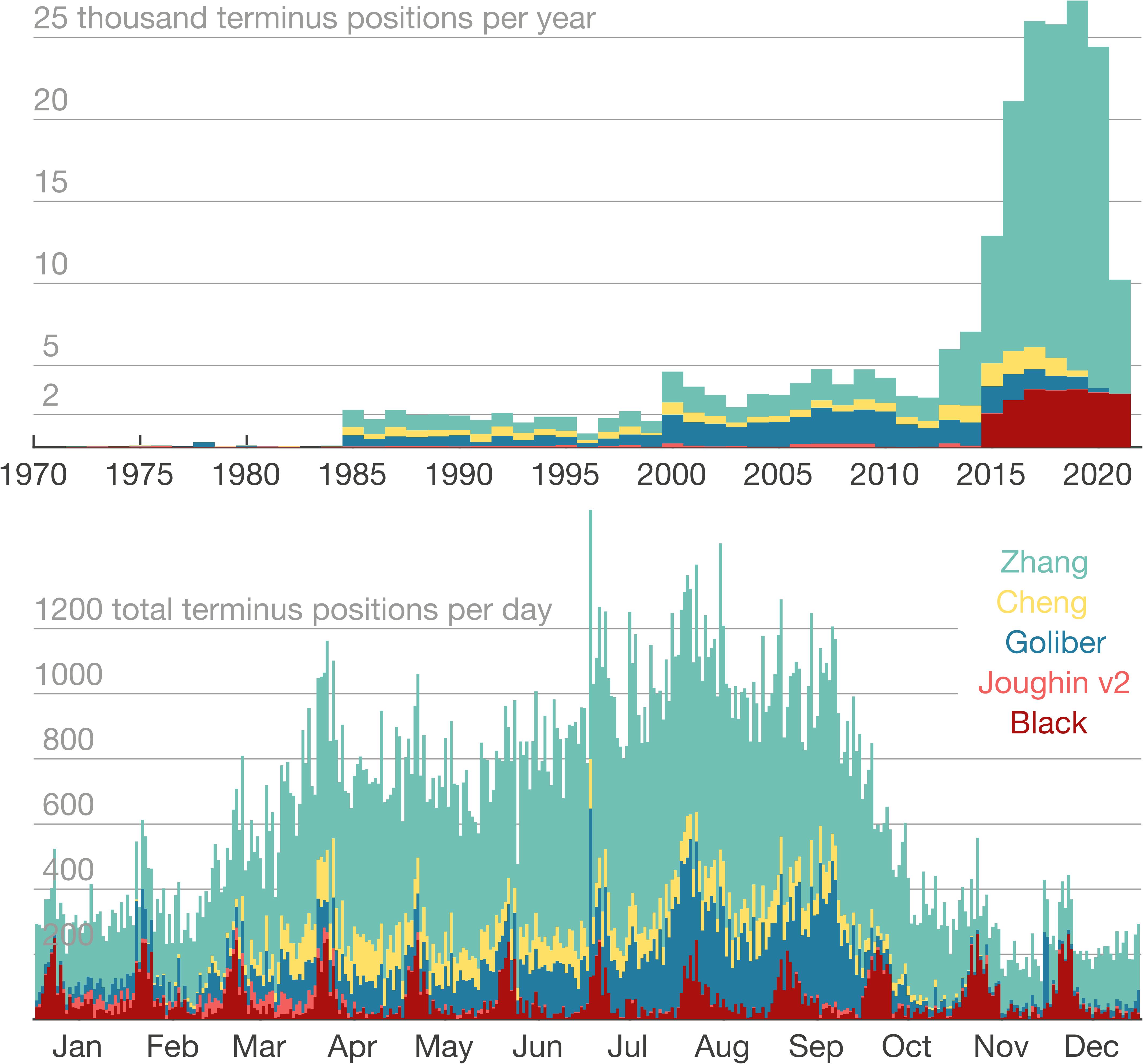
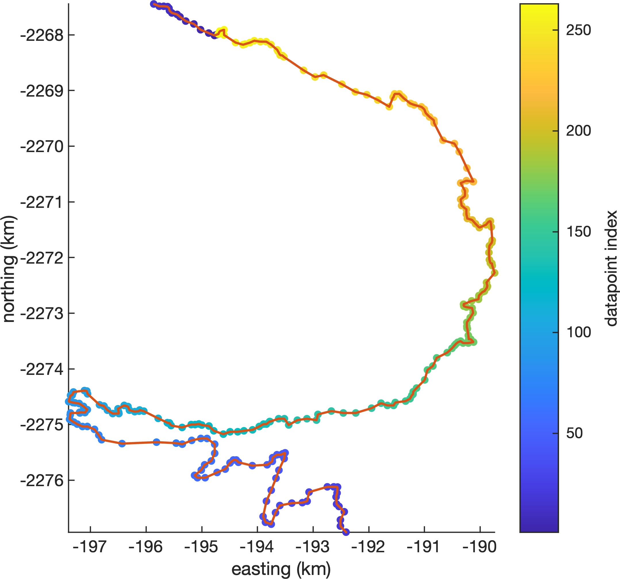
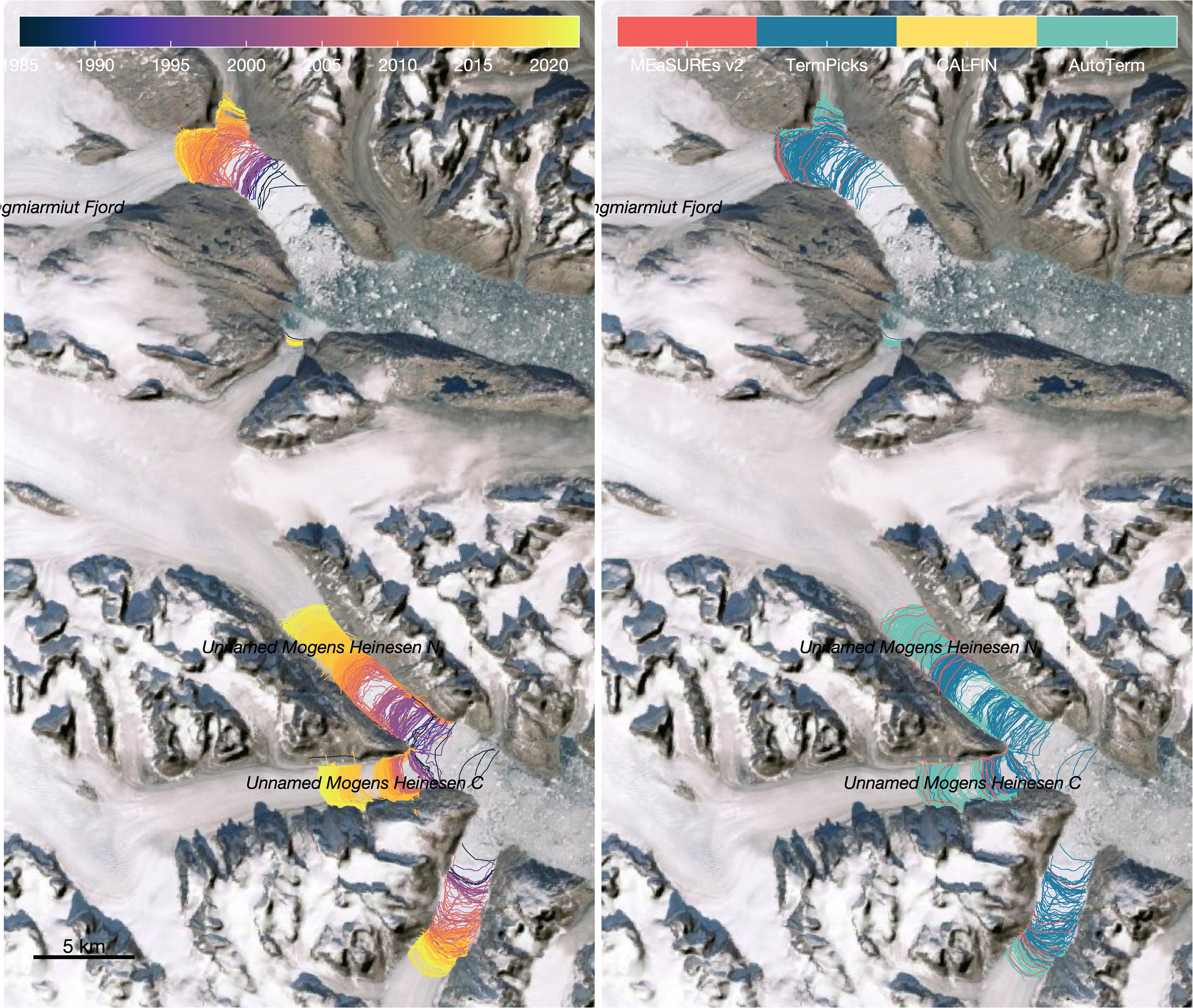
  c. Saves terminus_data_densified_2023-01-09.mat, which contains the densified terminus data as four simple columns of scattered data where x and y are polar stereographic meters, t is datenum, and p is a measure of data quality based on data sources and data quality flags, with highest numbers being the presumed best data. Here are a couple examples of the data created by terminus_data_densifier.m: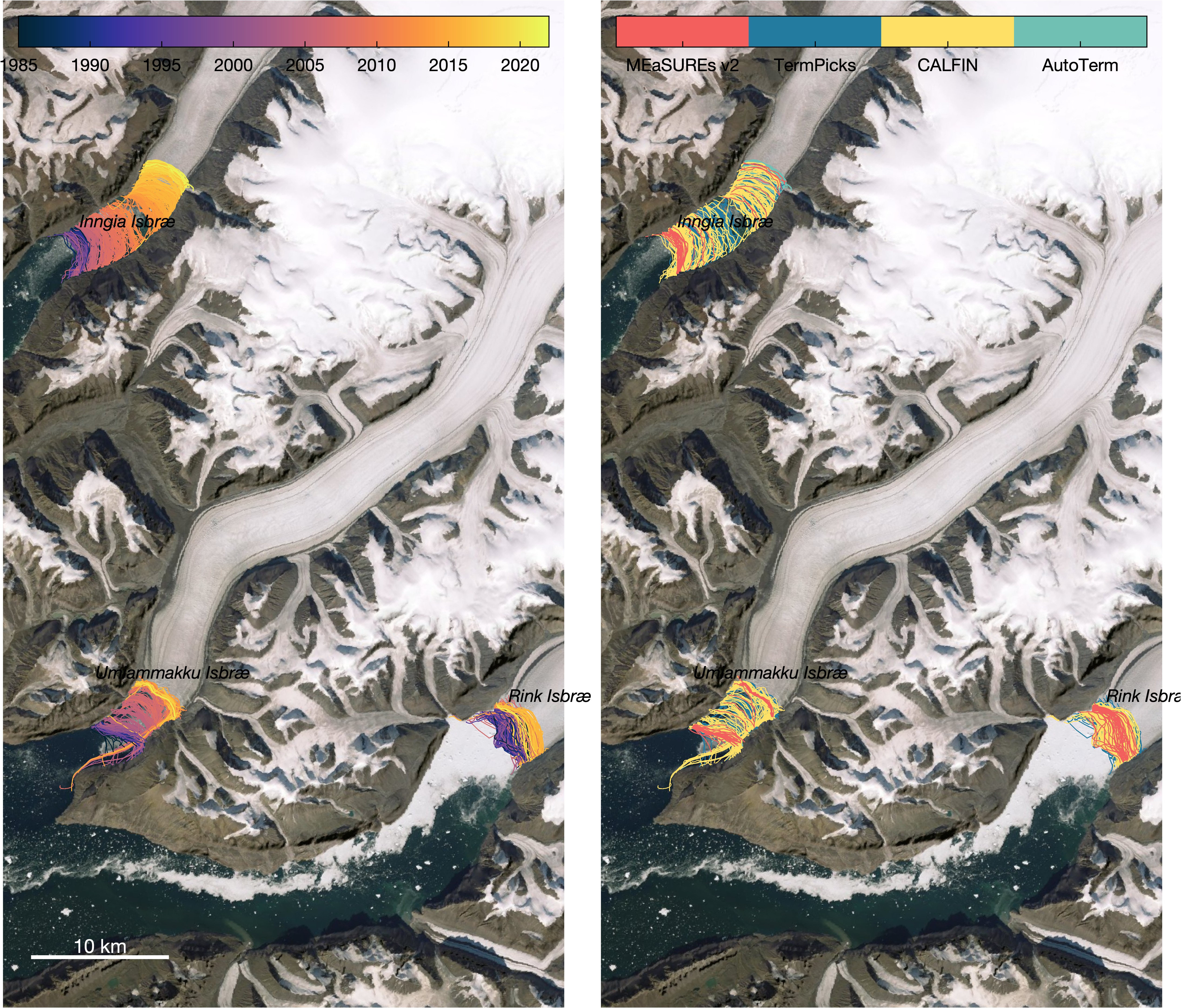
- Requirements:
  - export_fig (can be easily replaced by MATLAB's built-in exportgraphics function).
  - measures_greenland_terminus_picks_v2.mat created by measures_terminuspicks_compiler.m described above,
  - MATLAB's Mapping Toolbox (for shaperead and polyjoin),
  - Climate Data Toolbox for MATLAB for subsubplot and hline (can be replaced by built-in subplot and yline),
  - Arctic Mapping Tools for MATLAB for psnpath.
greenland_termini_to_icemasks.m creates monthly masks from terminus_data_densified.mat.
- This script loads densified terminus position data and gridded, extruded thickness & velocity data.
- The logic of the masking is as follows:
  
  a. Start with a gridded coastline from GimpOceanMask_90m_2015_v1.2.tif, which is a mosaic mask with a mean date of August 2015.
  
  b. Starting with time posting 2015-08-15: Find all terminus positions observed 30 days or fewer before 2015-08-15. Artifically advect them forward in time to their expected positions on 2015-08-15 and carve from the ice sheet everything downstream of the advected positions, as we assume the ice sheet didn't suddenly grow at a rate much faster than its average velocity.
  
  c. Find all terminus positions up to 30 days after 2015-08-15, artifically advect them upstream to their expected positions on 2015-08-15, and fill and set all pixels upstream of the advected terminus positions to true.
  
  Steps b and c are shown above for August 15, 2015. The ice mask is shown in white, starting with a Prior mask taken from GIMP 2015. The blue lines show all terminus observations taken within 30 days after 2015-08-15, but they have been advected upstream (using the extruded velocity grid) to their expected location on 2015-08-15. a. All pixels upstream of the blue lines are in the "Fill Region" and are set as true in the ice mask. Terminus positions observed within 30 days before 2015-08-15 are advected downstream to their expected location on 2015-08-15 (shown in yellow) and b. pixels downstream of the yellow line defined as being in the "Carve region" and are set as false in the ice mask. c. No adjustments are made where the Prior mask terminus falls between the Carve region and the Fill region. This can occur when ice is lost to calving in the time between terminus observations, or it can be due to a mismatch in terminus position picks. d. We set ice pixels to true wherever downstream-advected and upstream-advected terminus positions overlap.
  
  d. Use the adjusted mask created above as the basis for next month's ice mask and repeat steps b and c. Repeat until the last month of terminus position data.
  
  e. Repeat step d, but going backward, one month at a time, until the first month of terminus position data.
  
  f. Steps a-e make small adjustments to the ice mask only where observations disagree with the Prior mask. In months without direct observation, we assume that the ice front can only advance at a maximum rate given by the extruded ice velocity grid. We therefore start with the ice mask grid of penultimate month of our data cube (after performing steps a-e), we advect the grid cell center locations forward by one month and interpolate the last month's grid at the advected locations to determine which grid cells must have been ice in the penultimate month. We set them to true in the penultimate month and repeate the process for the previous month until we reach the first month in our data cube.
  
  g. As a result of step f, an erroneous seaward terminus pick can impact the ice mask for several months before the date of the erroneous observation. Or, the assumption of constant velocity may be inaccurate. In either case, it is possible that step f can overwrite some of this month's pixels based on next month's bad data. To ensure the best possible agreement between our final ice mask and the observations acquired in any given month, we repeat steps b-c for each month, using the data from each month after step f as the Prior ice grid.
- Requirements:
  - gridbin, which efficiently bins scattered data into a 2D grid.
  - filt2 from Climate Data Toolbox for MATLAB to lowpass filter the GIMP mask before interpolating.
greenland_icemask_animations_for_qc.m creates glacier-by-glacier animations for quality control checks. These animations plot the final icemask along with the glacier pick data that went into them.
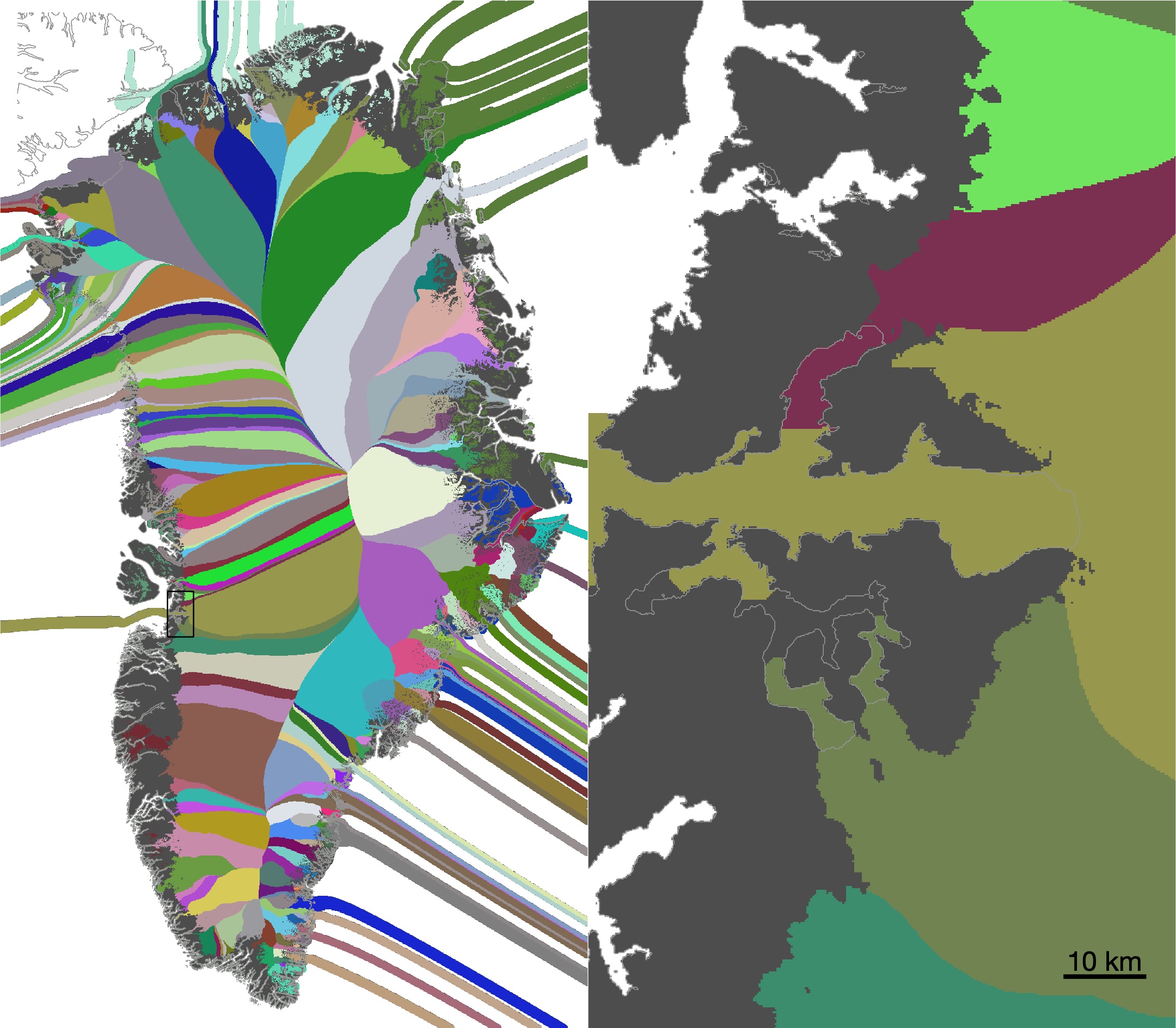
icemask_catchment_analysis.m creates icemask_catchment_analysis_1972-2022_v1.mat, which contains a time series of area and mass by basin for the entire ice sheet. This script is very inefficient and takes about two days to run.
ice_catchment_area_mass_timeseries_analysis.m analyzes the time series in icemask_catchment_analysis_1972-2022_v1.mat to quantify total area and mass changes on decadal and seasonal timescales. Also creates this plot: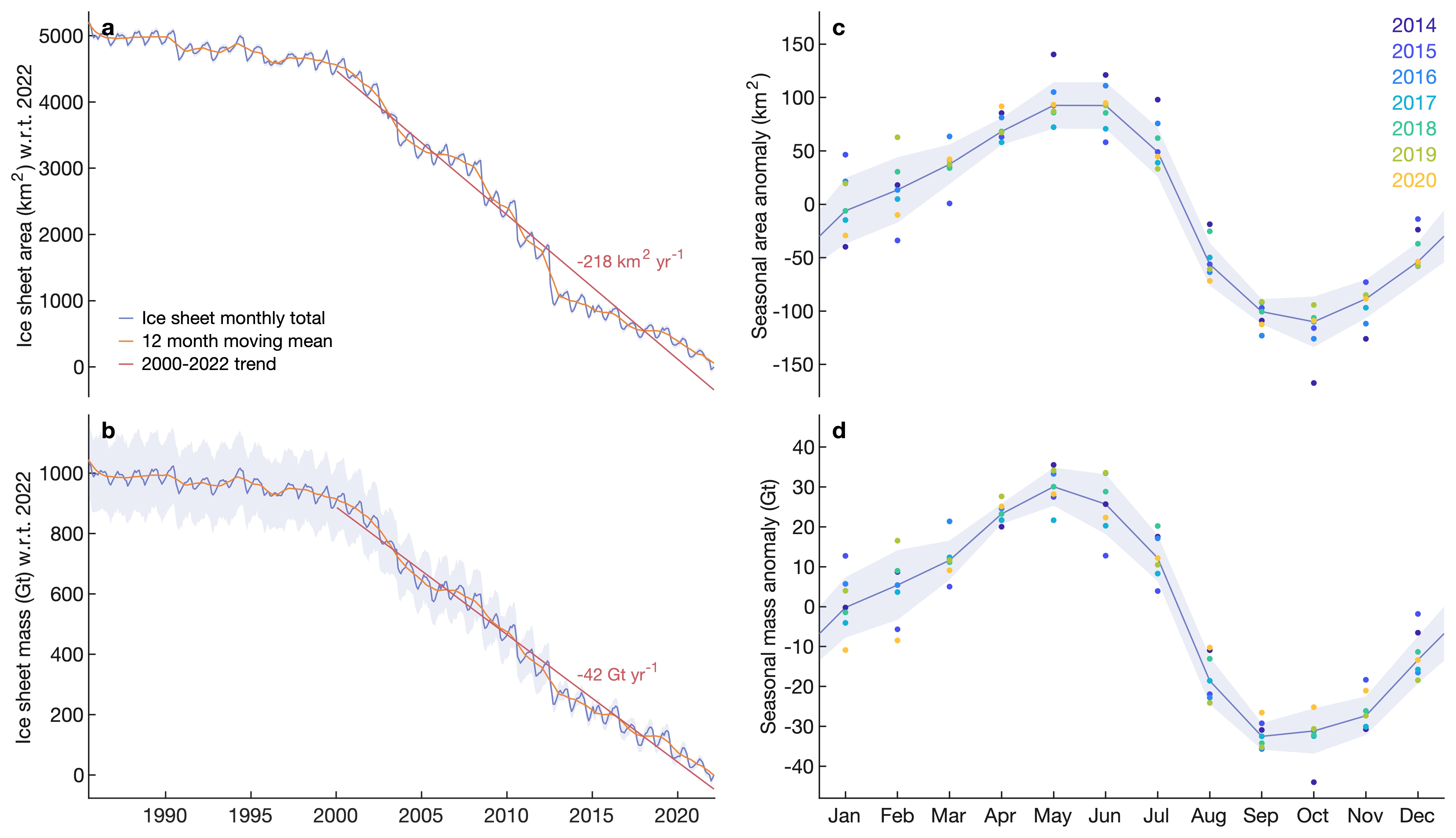

Functions

terminus_masker_advect performs the heavy lifting of synthetically advecting terminus positions upstream and downstream to create a time-evolving monthly mask.
remove_icebergs finds bits of ice that detach from the ice sheet, and removes them from a land mask cube.
stream2_fast is an edited version of Matlab's built-in stream2 function. The main difference is that stream2_fast doesn't waste time sorting input x and y coordinates (which accounts for about half of the processing time of stream2 the way it's used in this work.)

Quality control

Here's an animation of the final product:

Ruitao-Terry / greenland-icemask