10th (currently 7th place while leaderboard is being updated) place solution for the 2018 Data Science Bowl with a score of 0.591 with a single model submission.
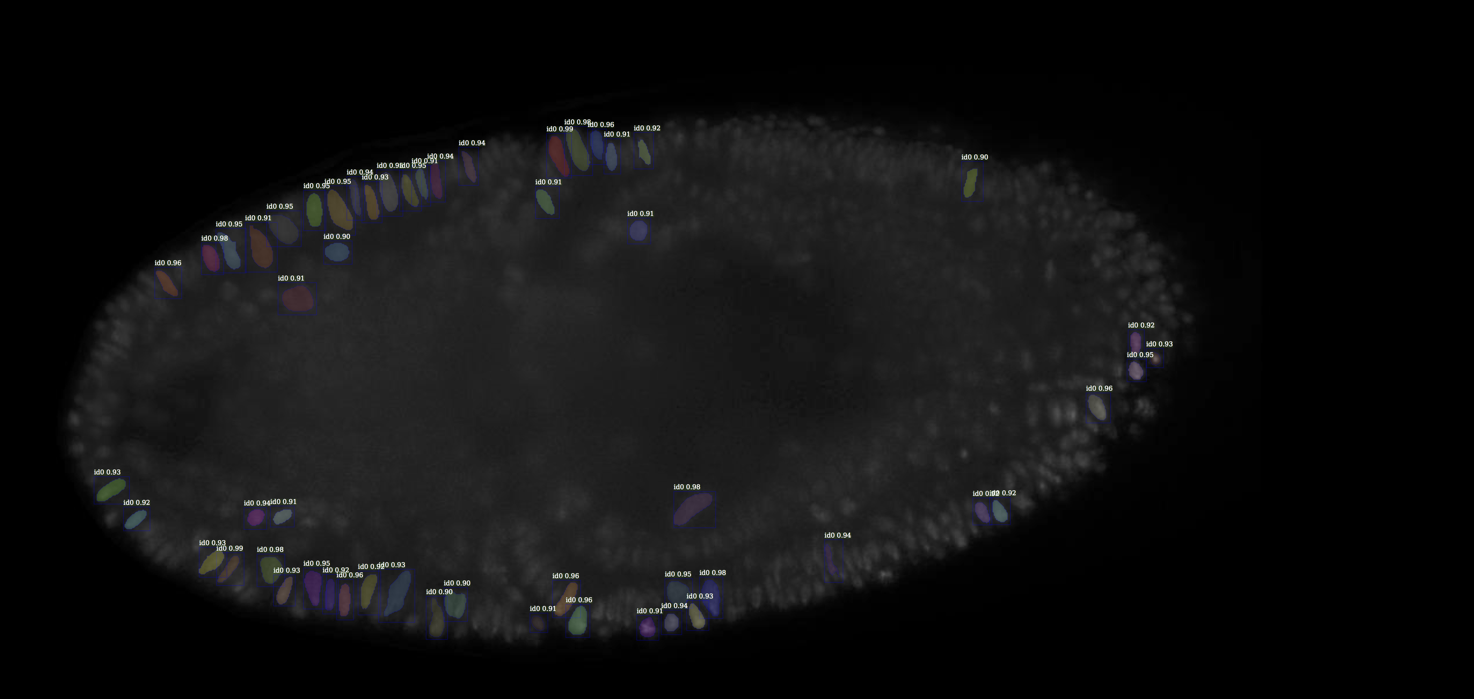
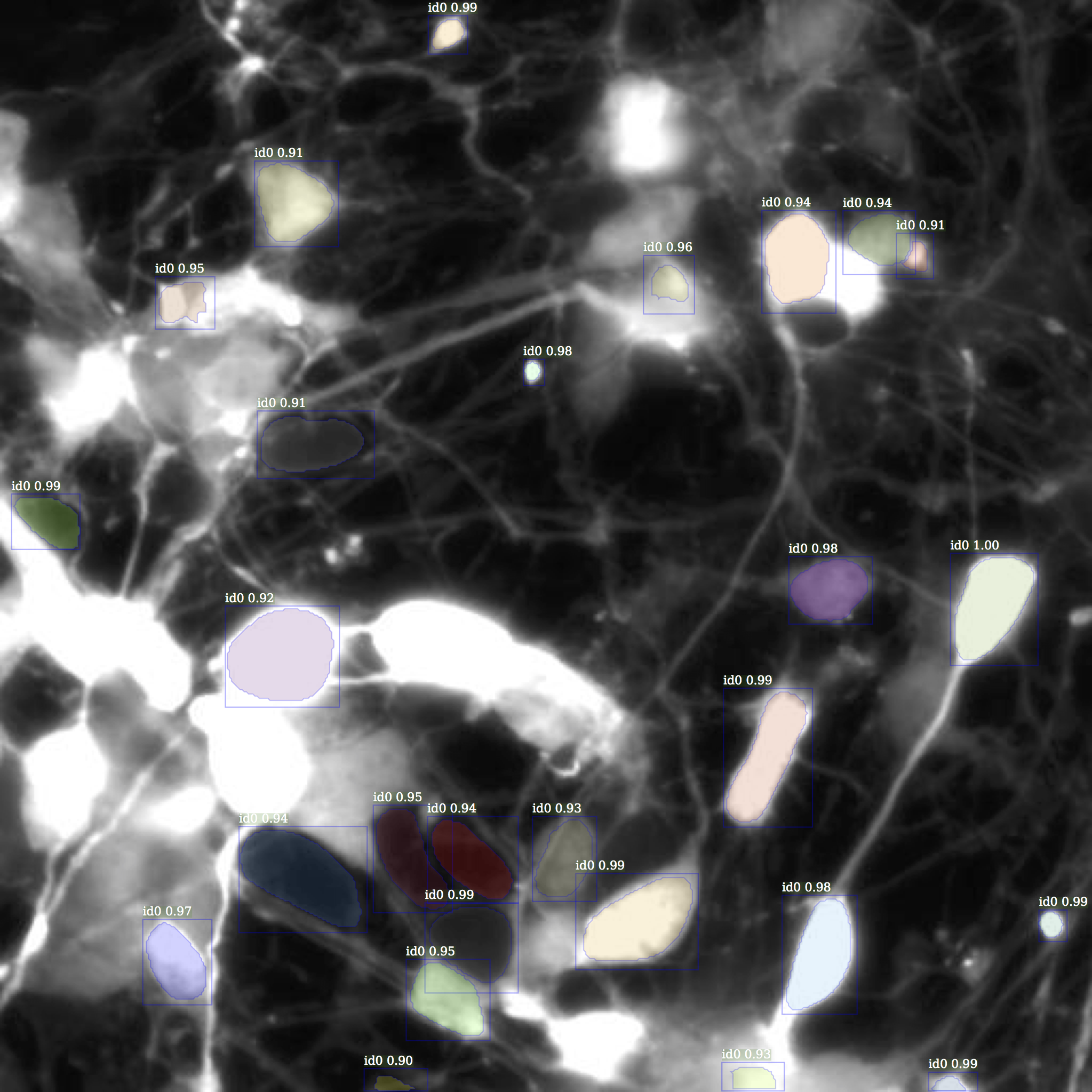
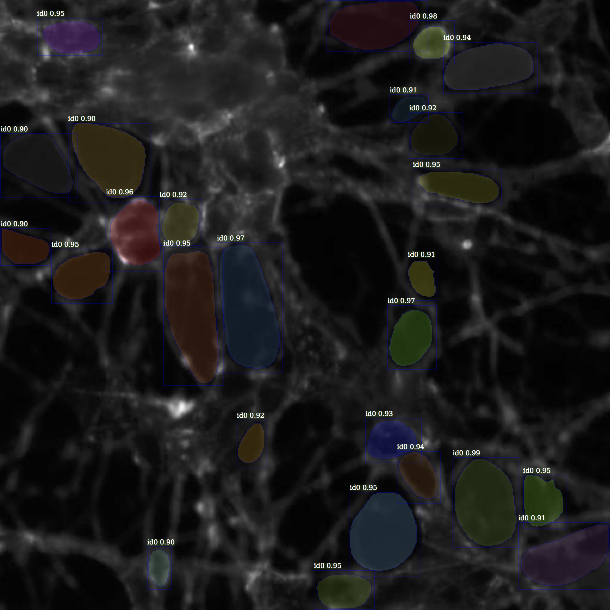
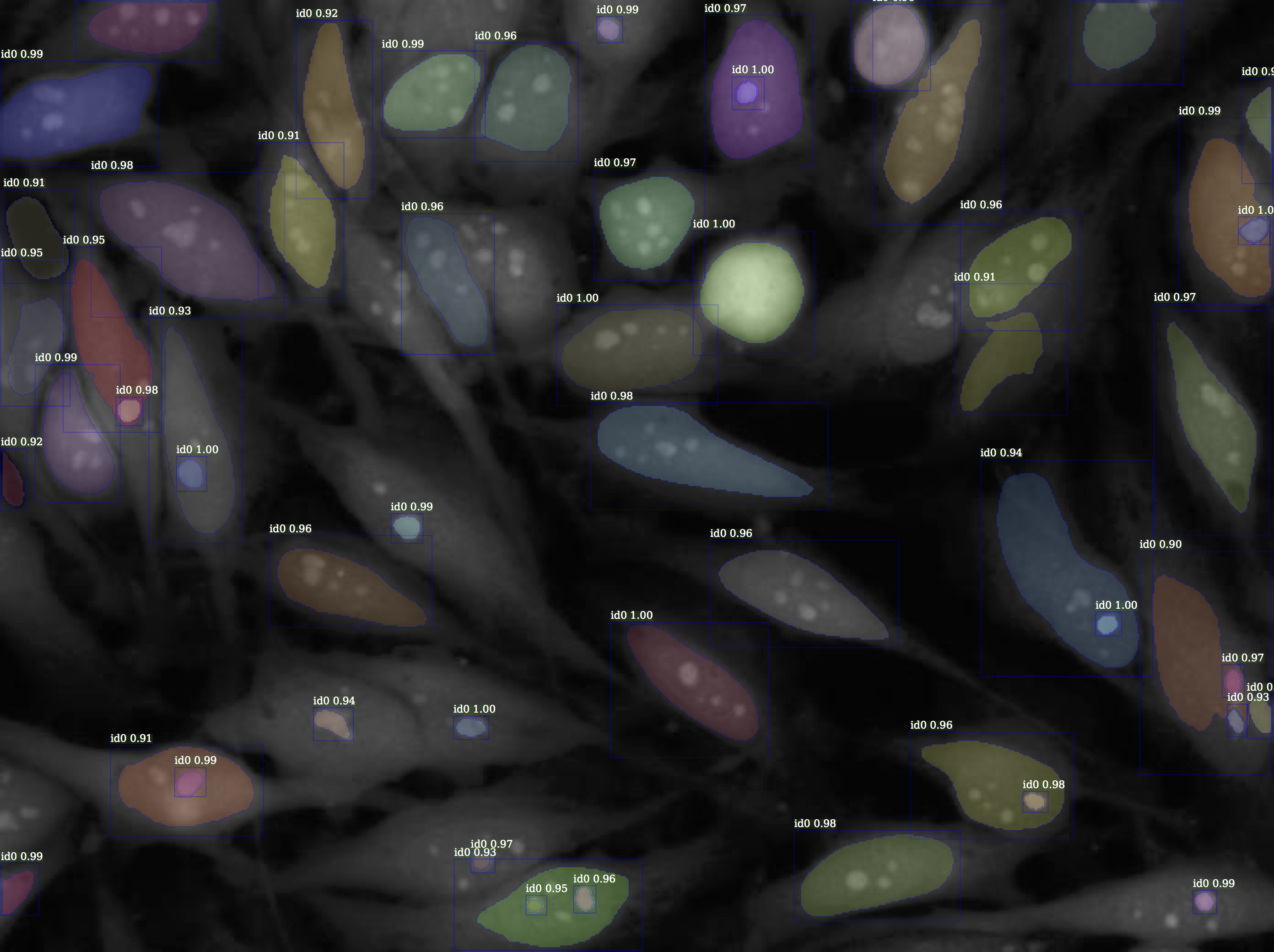
Nuclei Detectron is built on Detectorn which is a Mask R-CNN based solution. This approach was chosen since Mask R-CNN works well on instance segmentation problems.
P.S. Unofficial score of 0.608 without ensemble on submissions that were not in the 2 final submissions.
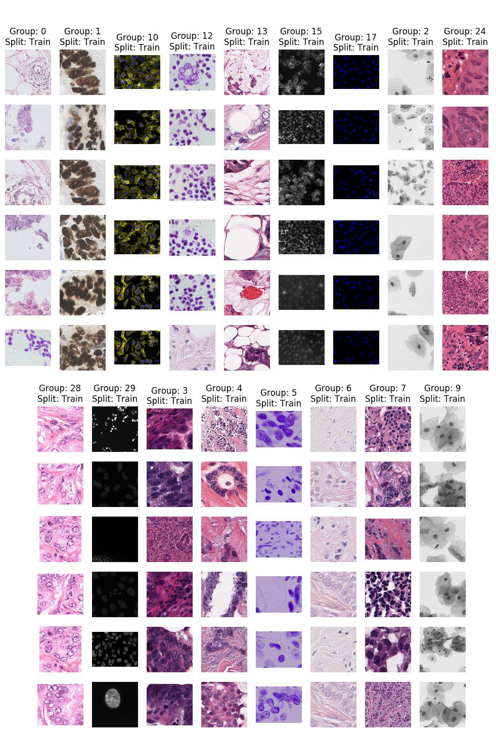
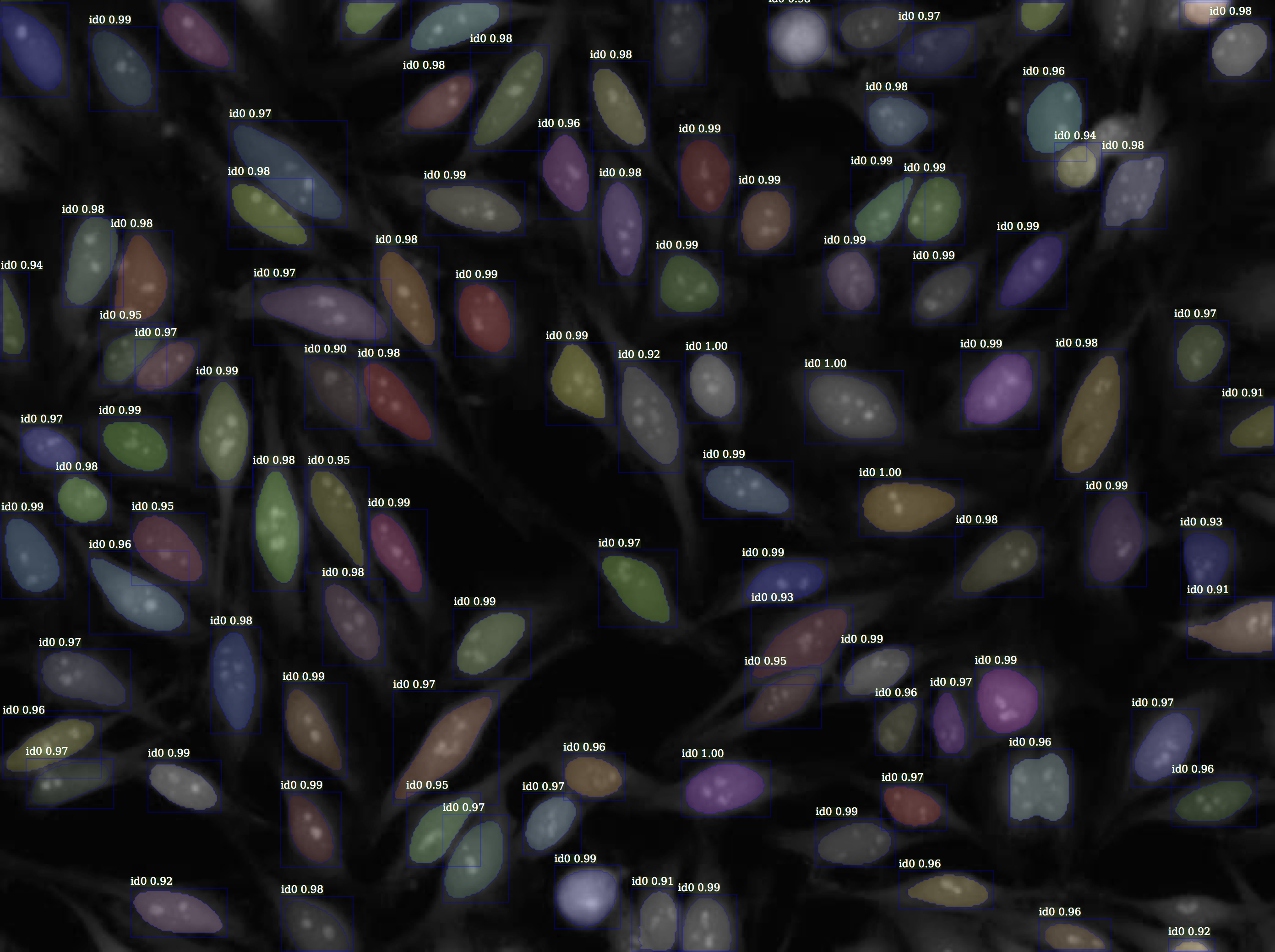
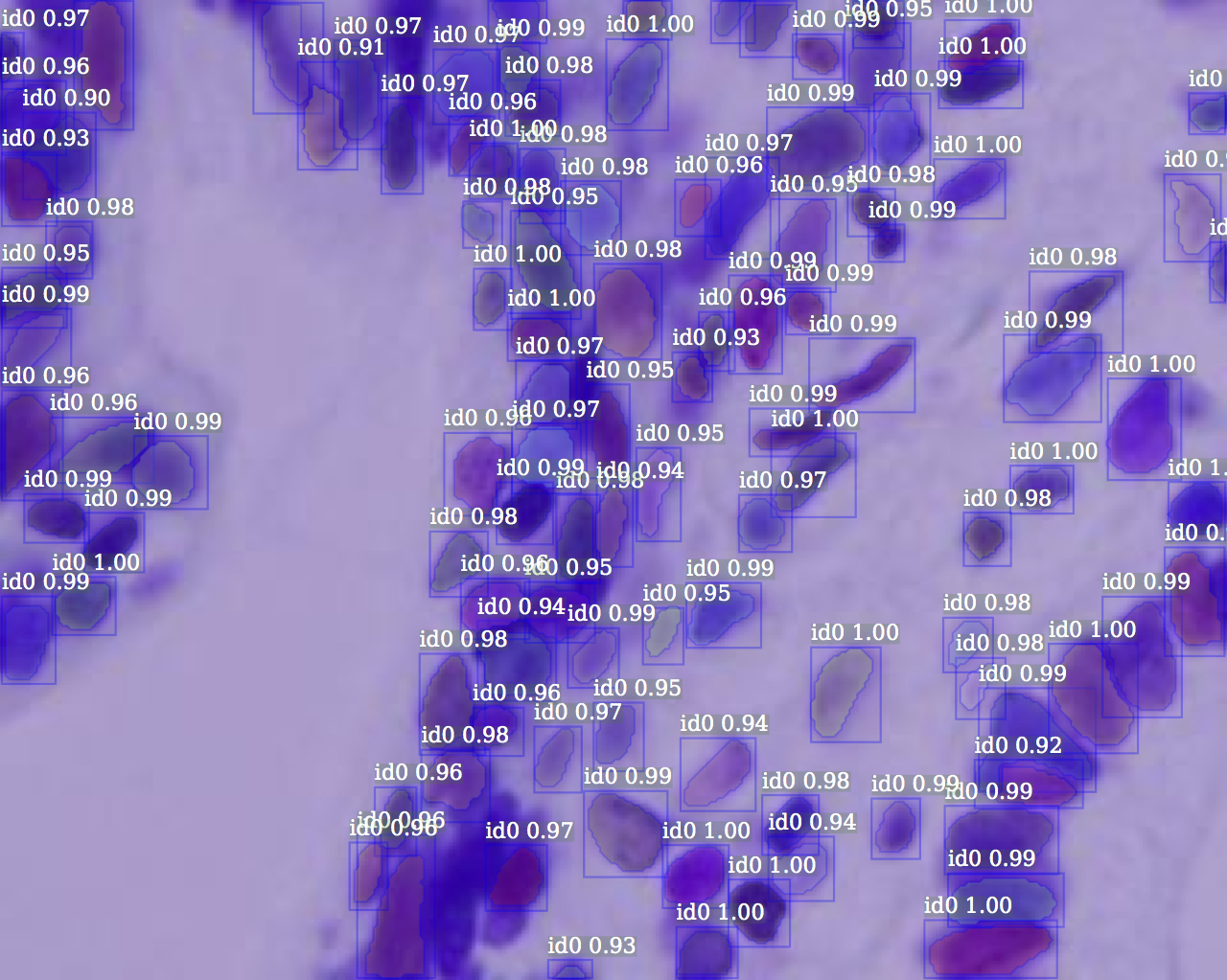
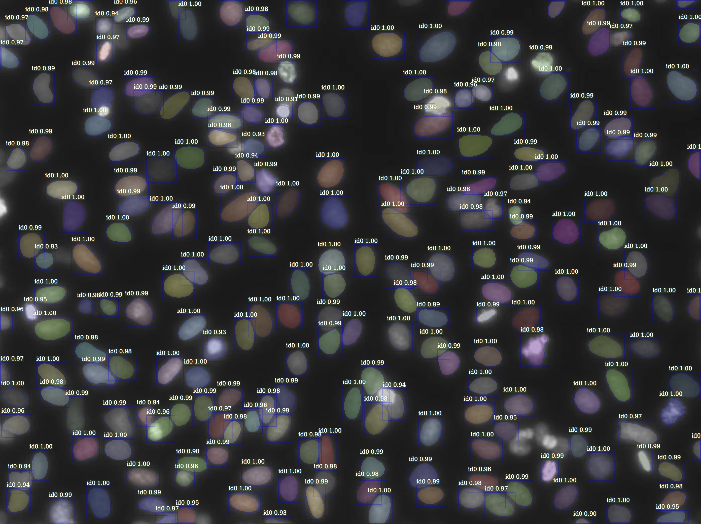
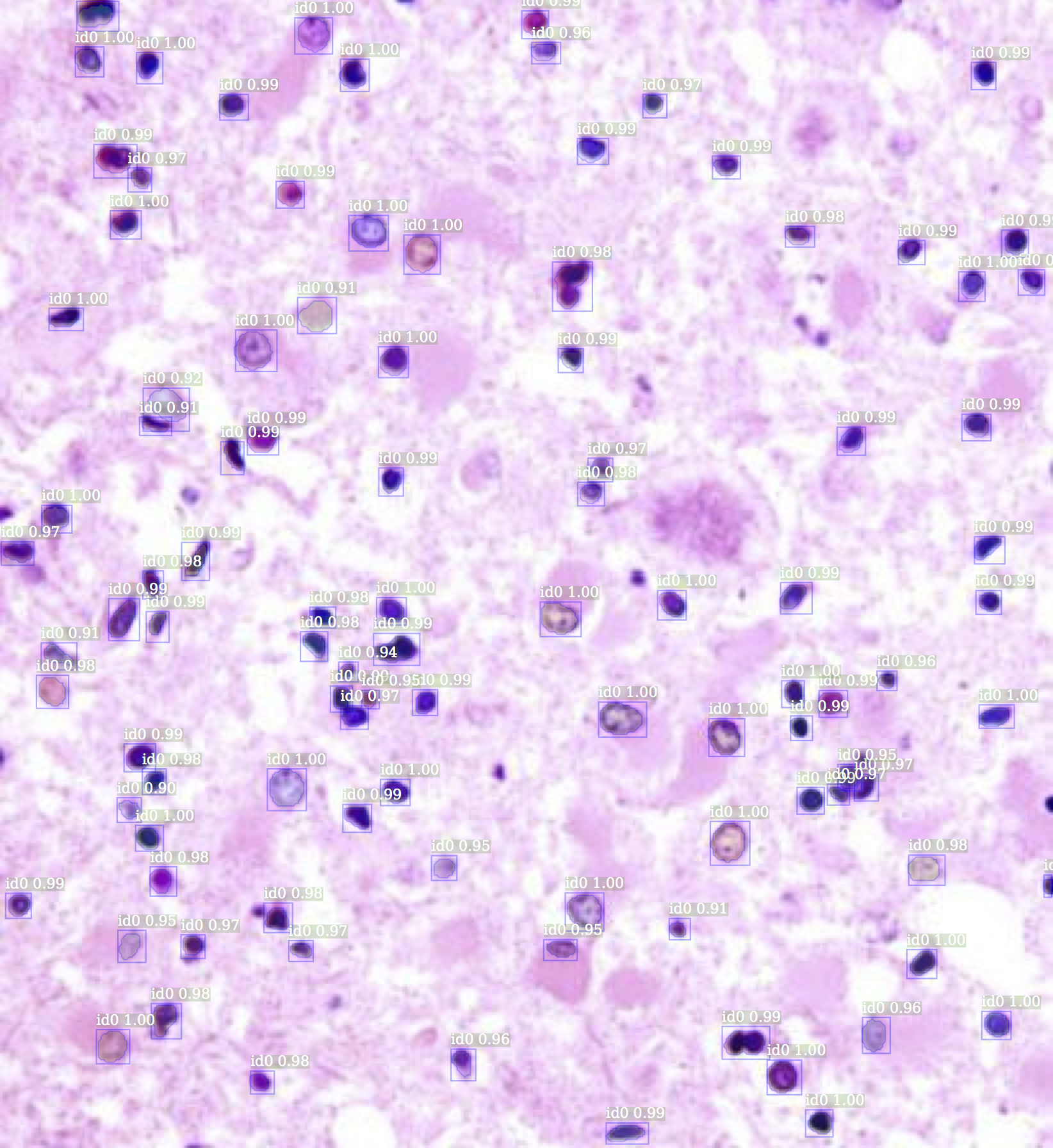
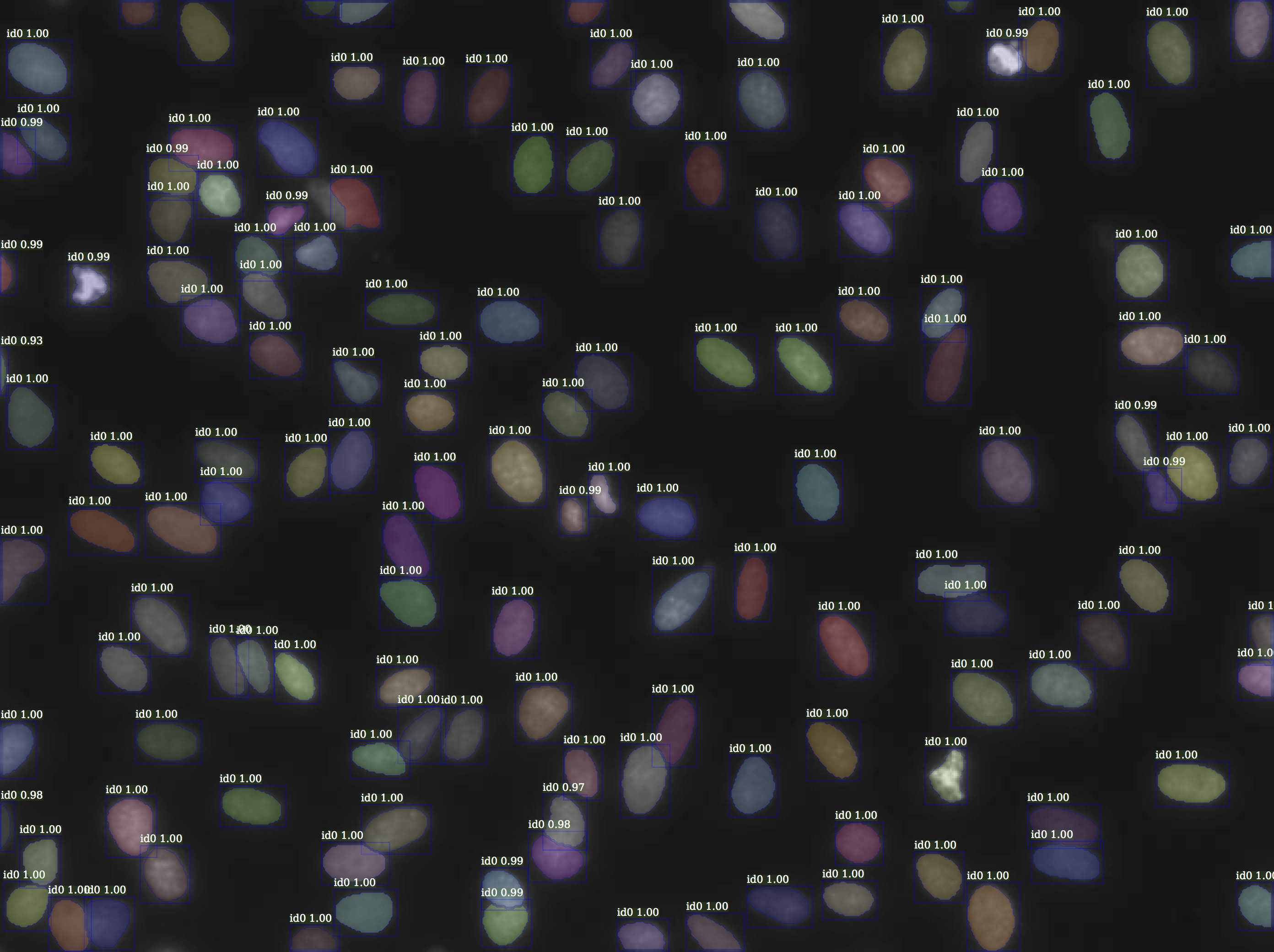
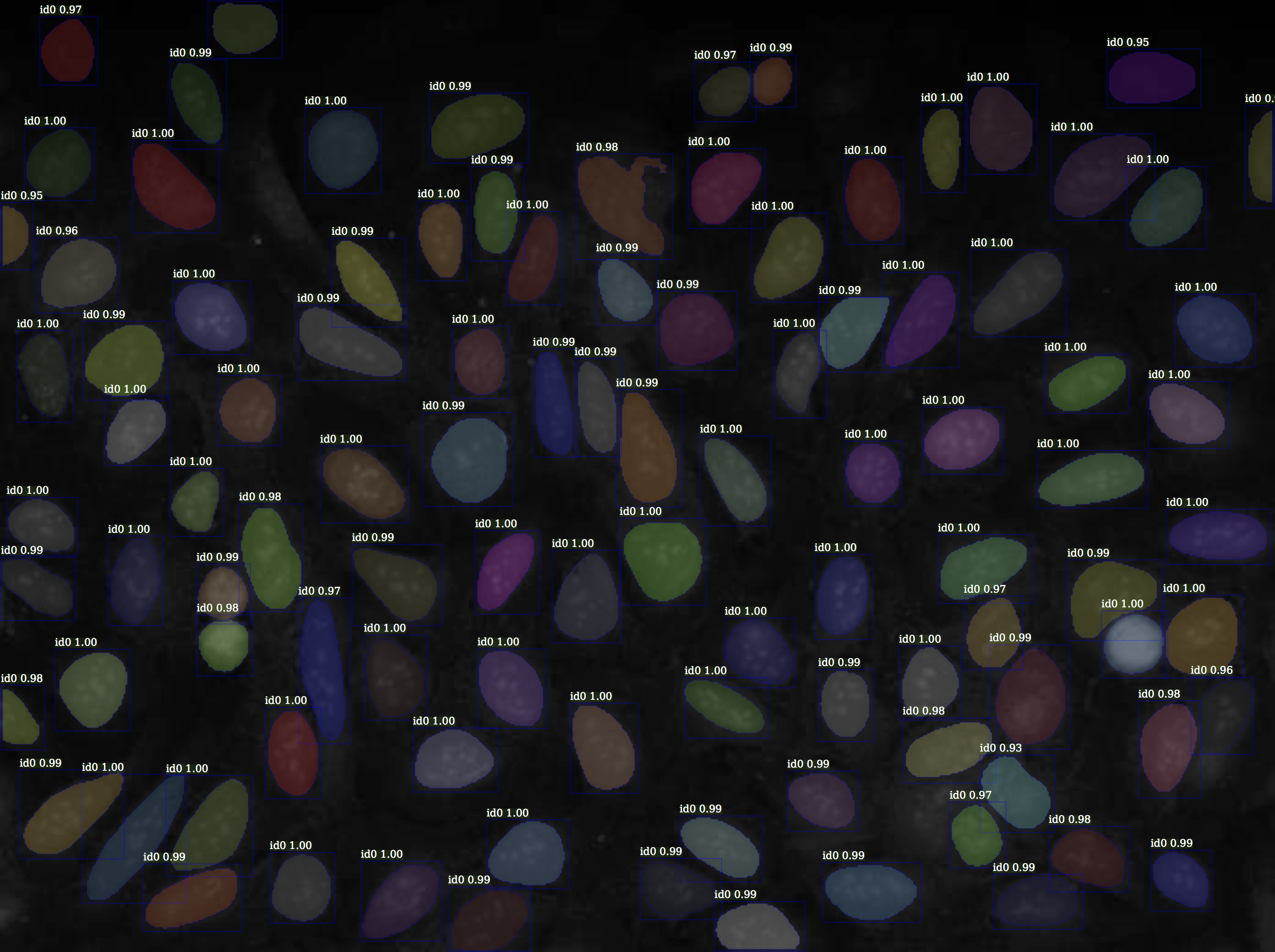
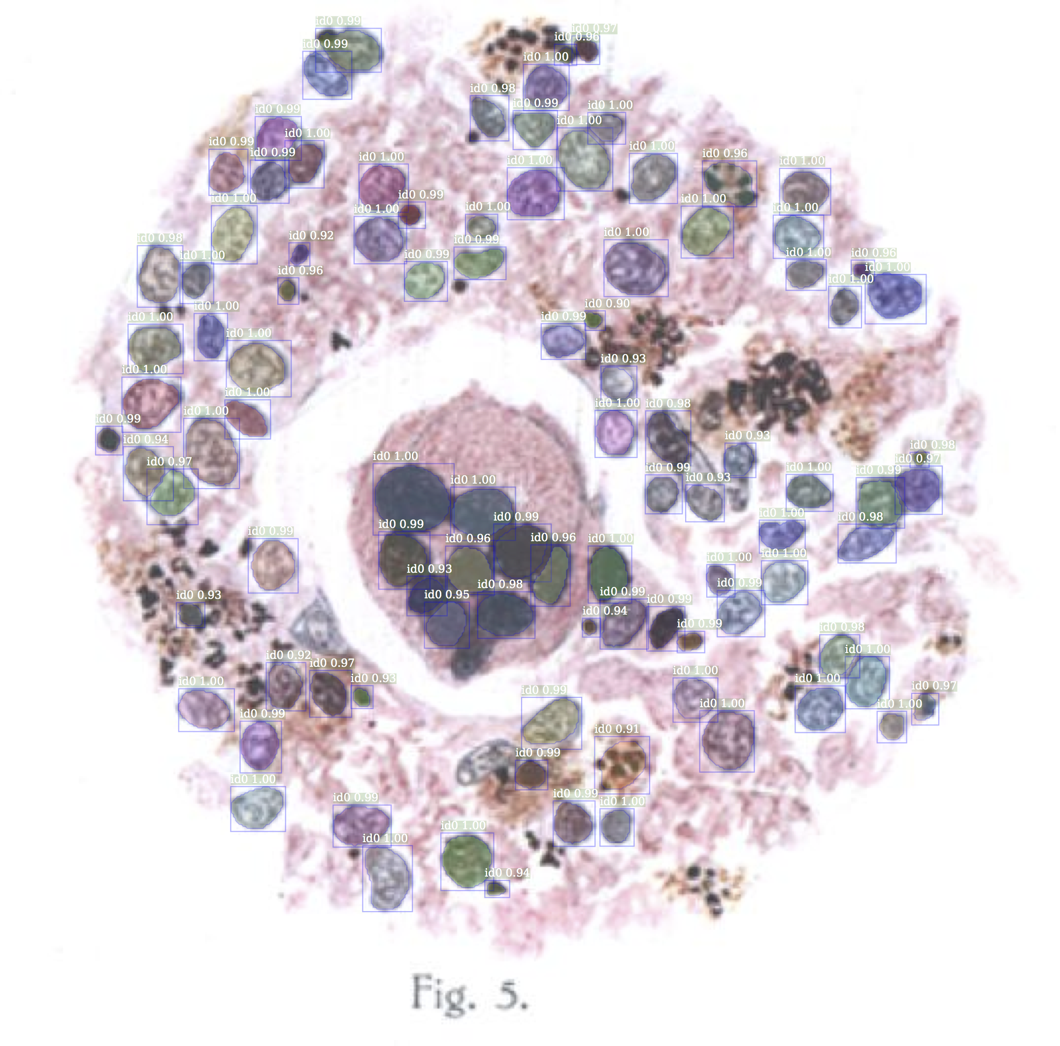
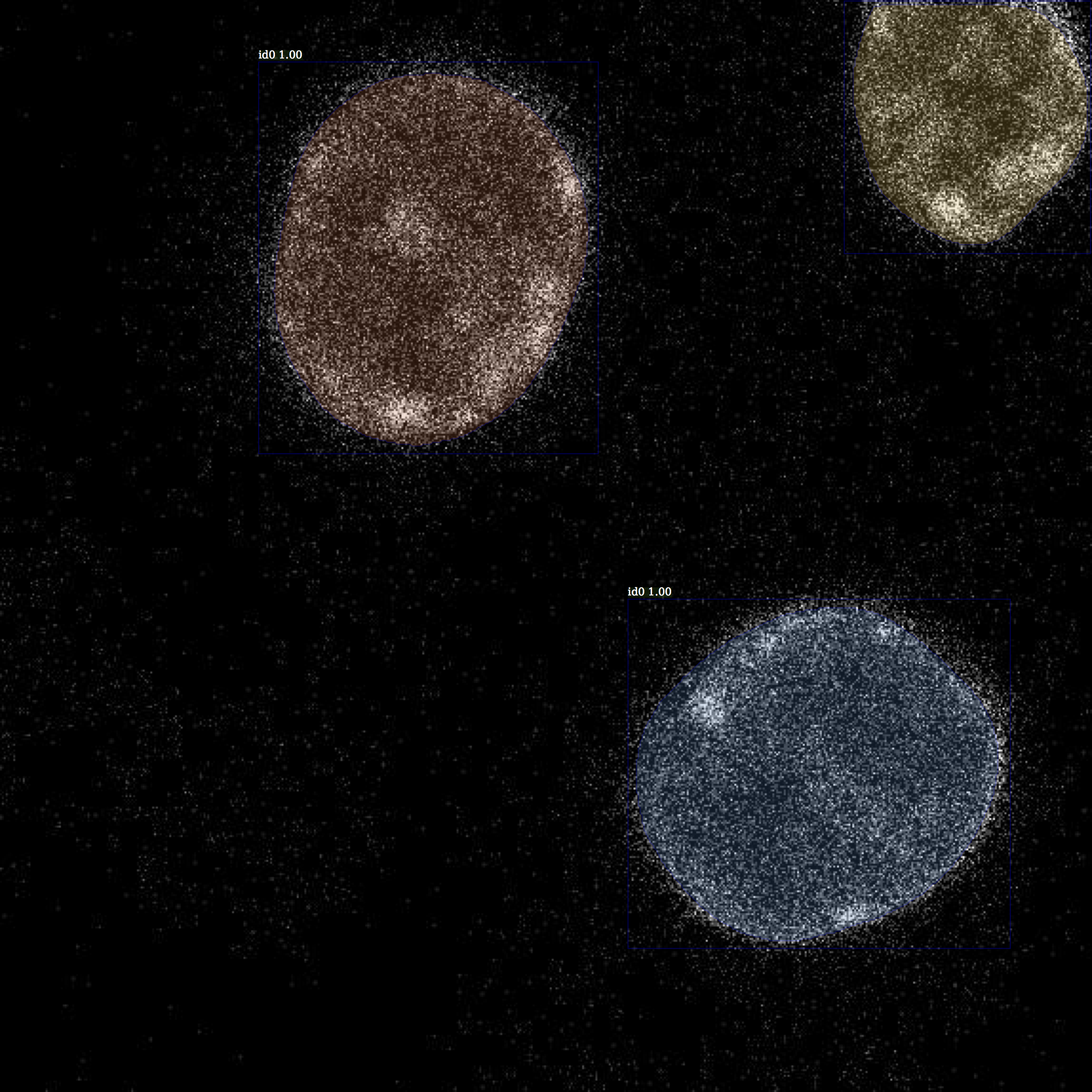
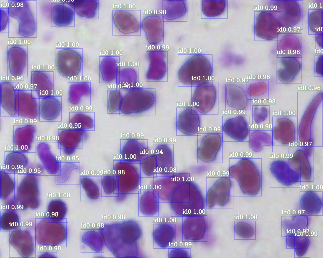
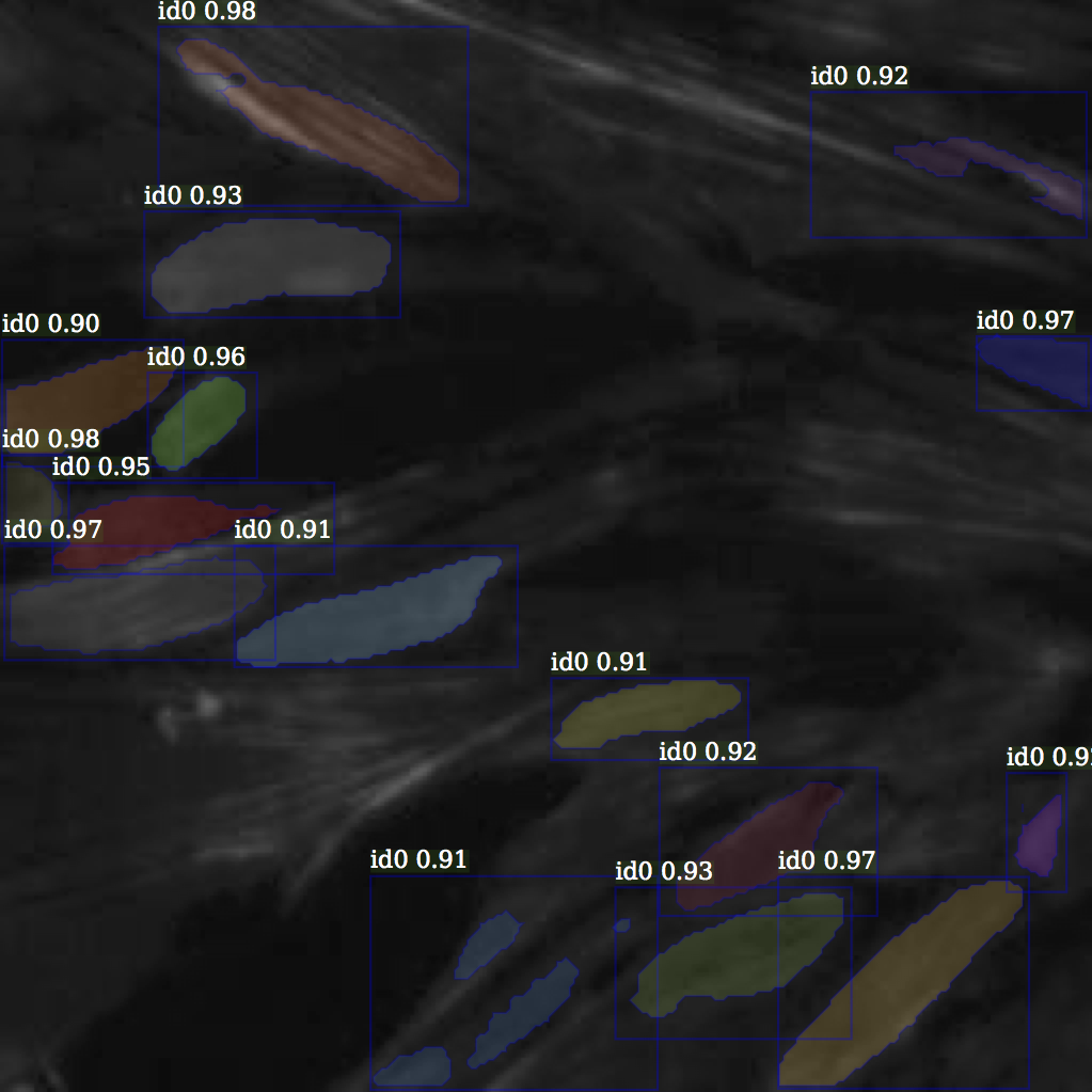
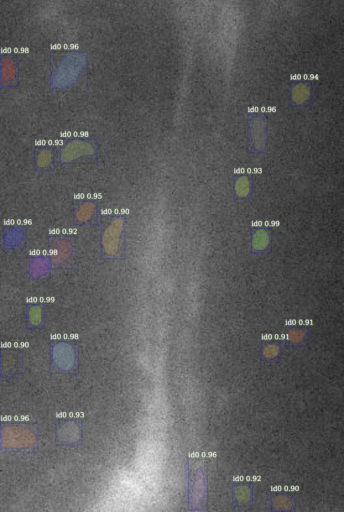
The challenge is to build a model that can identify a range of nuclei across varied conditions. The hard part of the challenge is to generalize across nuclei types that are very different from training set, and in different lighting conditions.
 |
 |
 |
 |
 |
 |
 |
 |
 |
 |
 |
 |
 |
 |
 |
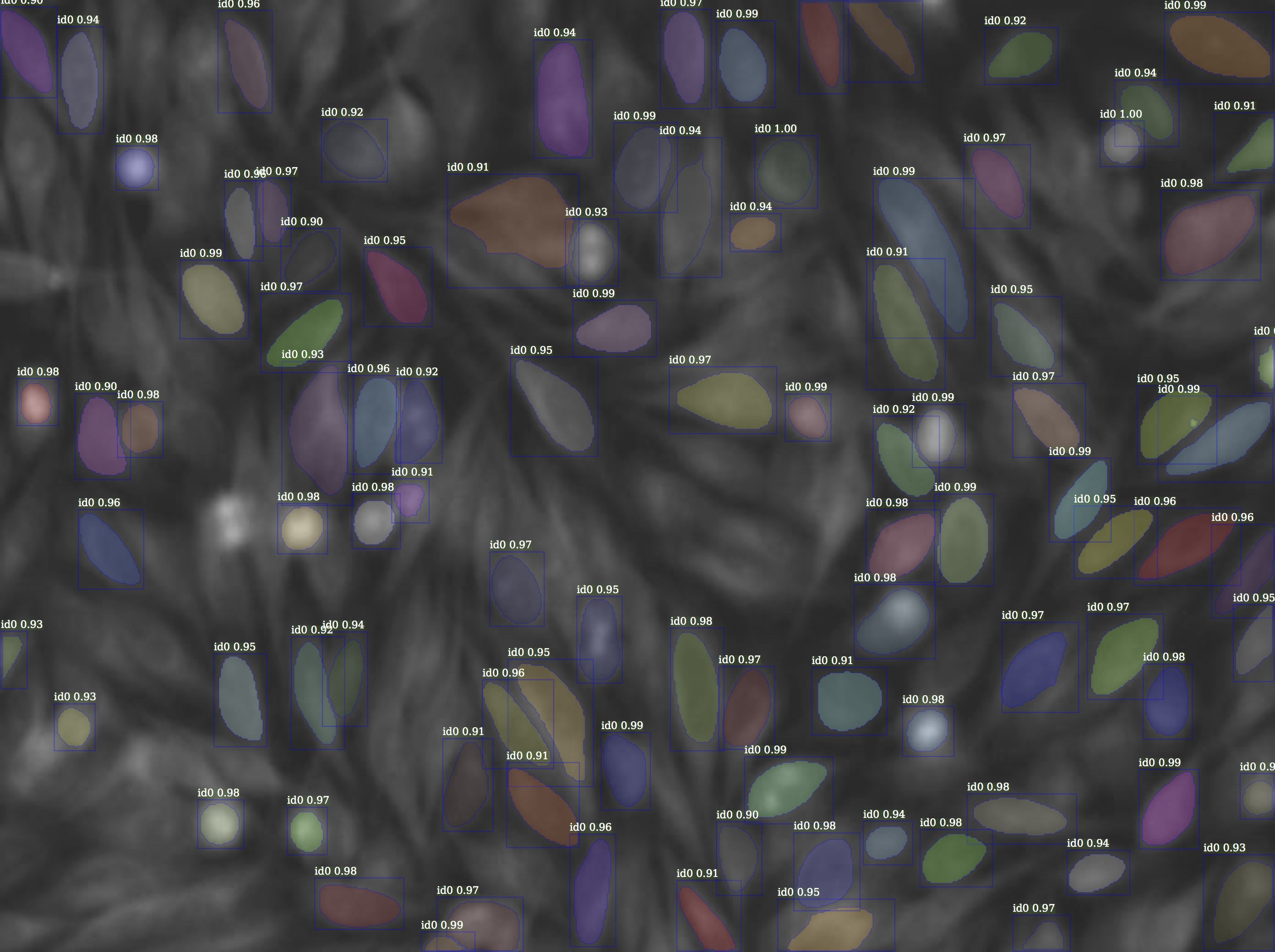 |
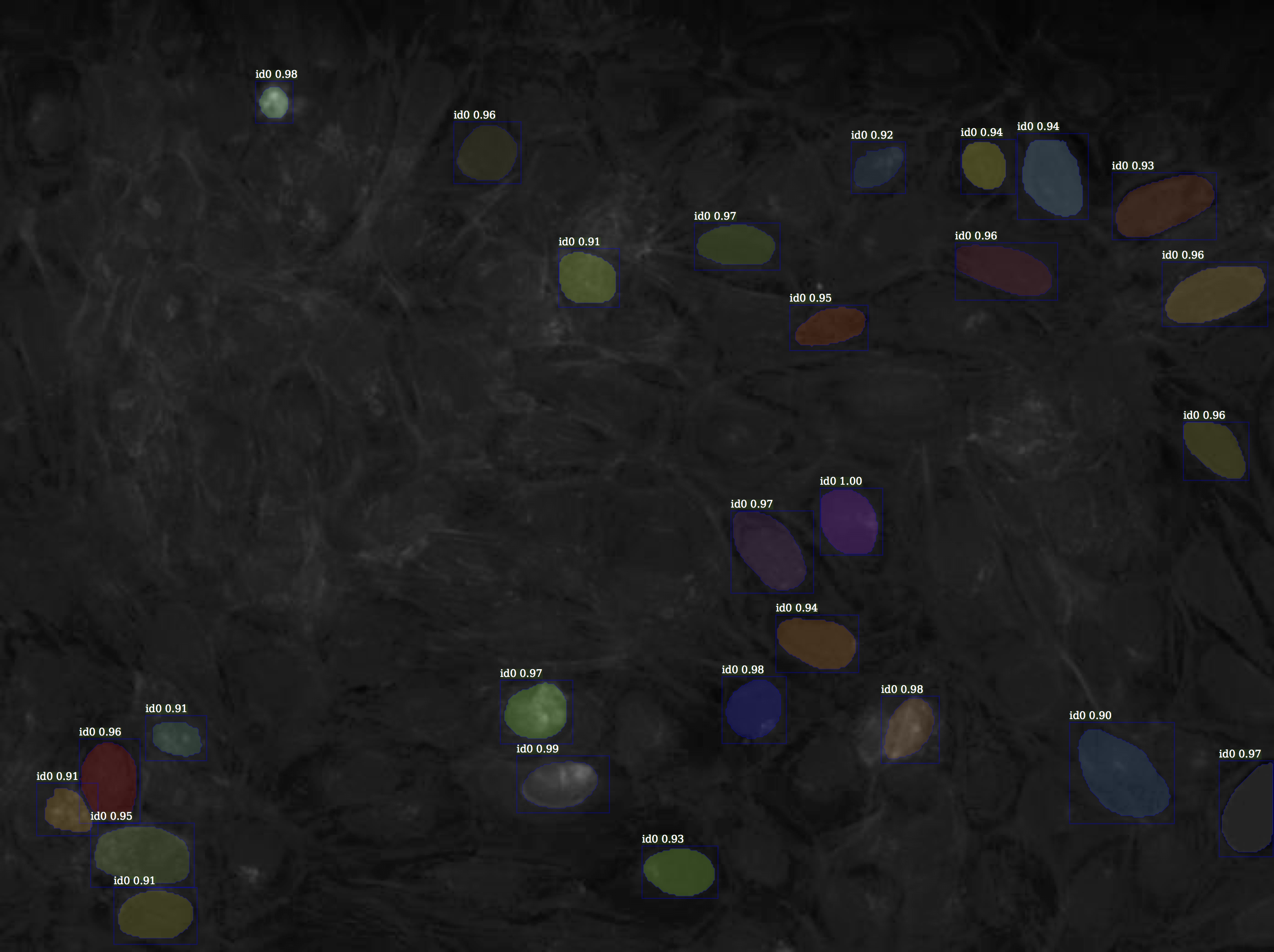 |
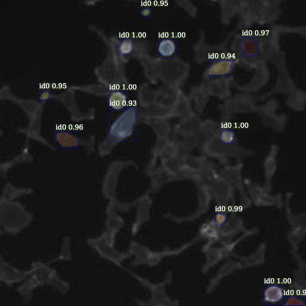 |
- There were several nuclei datasets with outlines as annotations.
- Applied classical computer vision techniques to convert ground truth from outlines to masks.
- This involved adding boundary pixels to the image so all contours are closed.
- Given outlines of cells with overlaps/touching or at border,
- Mark an outer contour to encompass contours that are at image edges.
- then do cv2.findContours to get the polygons of mask.
- Ref parse_segments_from_outlines
- Standardized all datasets into COCO mask RLE JSON file format.
- You can use cocoapi to load the annotations.
- Cut image into tiles when images are bigger than 1000 pixels
- This was necessary since large image features did not fit in GPU memory.
- Cluster images into classes based on the color statistics.
- Normalize classes size
- Oversample/undersample images from clusters to a constant number of images per class in each epoch.
- Fill holes in masks
- Split nuclei masks that are fused
- Applied morphological Erosion and Dilation to seperate fused cells
- Use statistics of nuclie sizes in an image to find outliers
- ZCA whitening of images
- Zero mean unit variance normalization
- Grey scale: Color-to-Grayscale: Does the Method Matter in Image Recognition.
- Very important how you convert to grey scale. Many algorithms for the conversion, loss of potential data.
- Luminous
- Intensity
- Value: This is the method I used.
- Contrast Limited Adaptive Histogram Equalization
Data augmentation is one of the key to achieve good generalization in this challenge.
- Invert
- This augmentation helped in reducing generalization error significantly
- Randomly choosing to invert caused the models to generalize across all kids of backgrounds in the local validation set.
- Geometric
- PerspectiveTransform
- This is very useful to make the circular looking cells to look stretched
- PiecewiseAffine
- Flip
- Rotate (0, 90, 180, 270)
- Crop
- PerspectiveTransform
- Alpha blending
- Create geometrical blur by affine operation
- Shear, rotate, translate, scale
- Pixel
- AddToHueAndSaturation
- Multiply
- Dropout, CoarseDropout
- ContrastNormalization
- Noise
- AdditiveGaussianNoise
- SimplexNoiseAlpha
- FrequencyNoiseAlpha
- Blur
- GaussianBlur
- AverageBlur
- MedianBlur
- BilateralBlur
- Texture
- Superpixels
- Sharpen
- Emboss
- EdgeDetect
- DirectedEdgeDetect
- ElasticTransformation
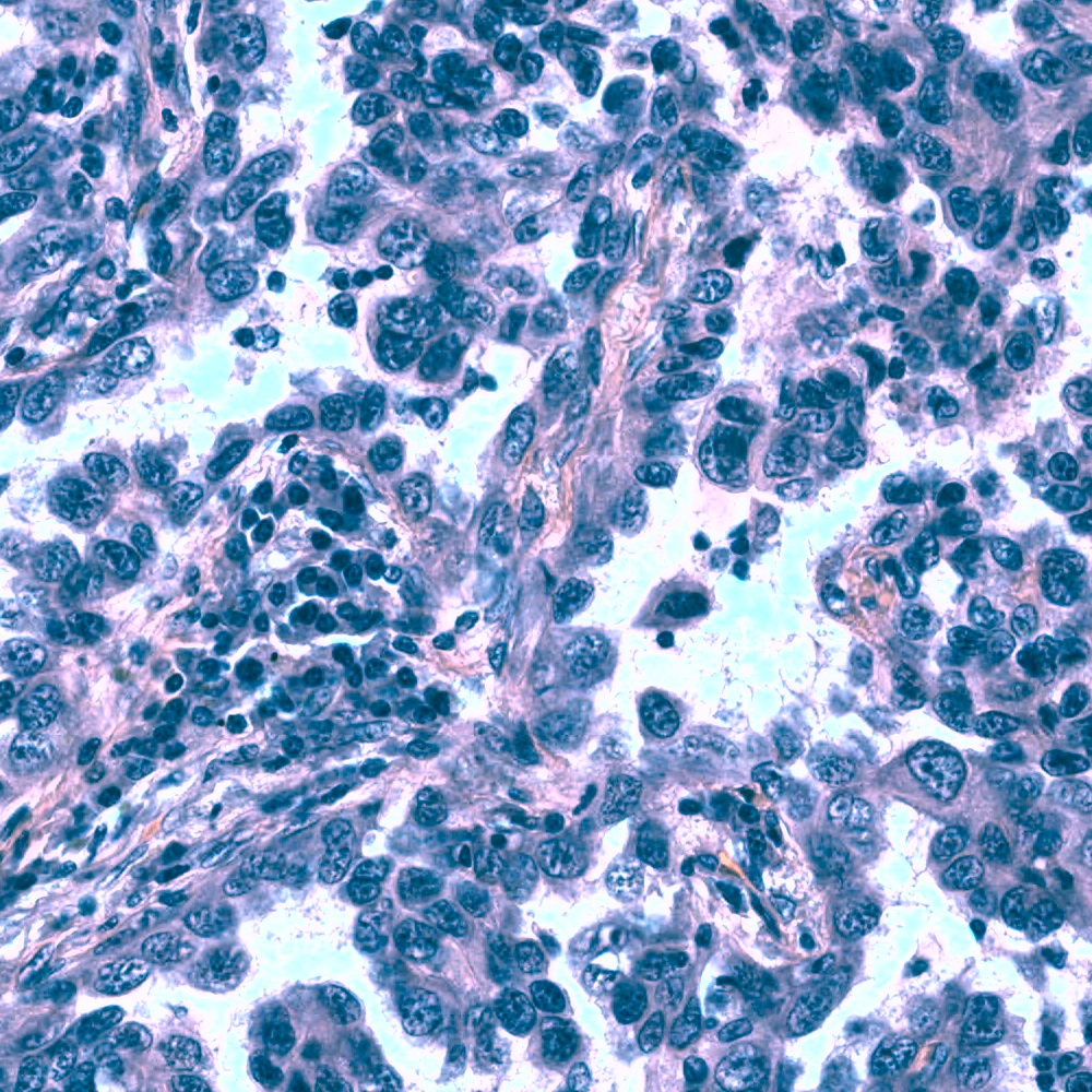
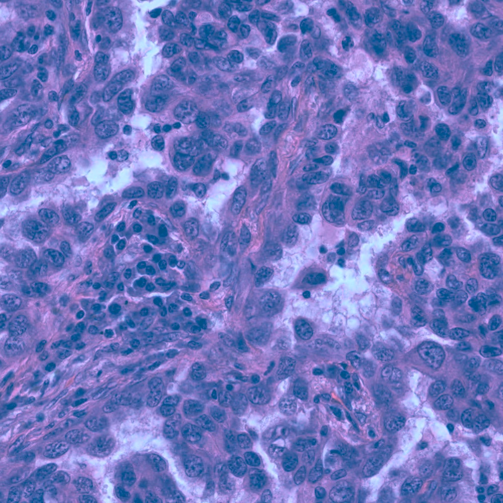
| Original Image | Random Augmentations for training |
|---|---|
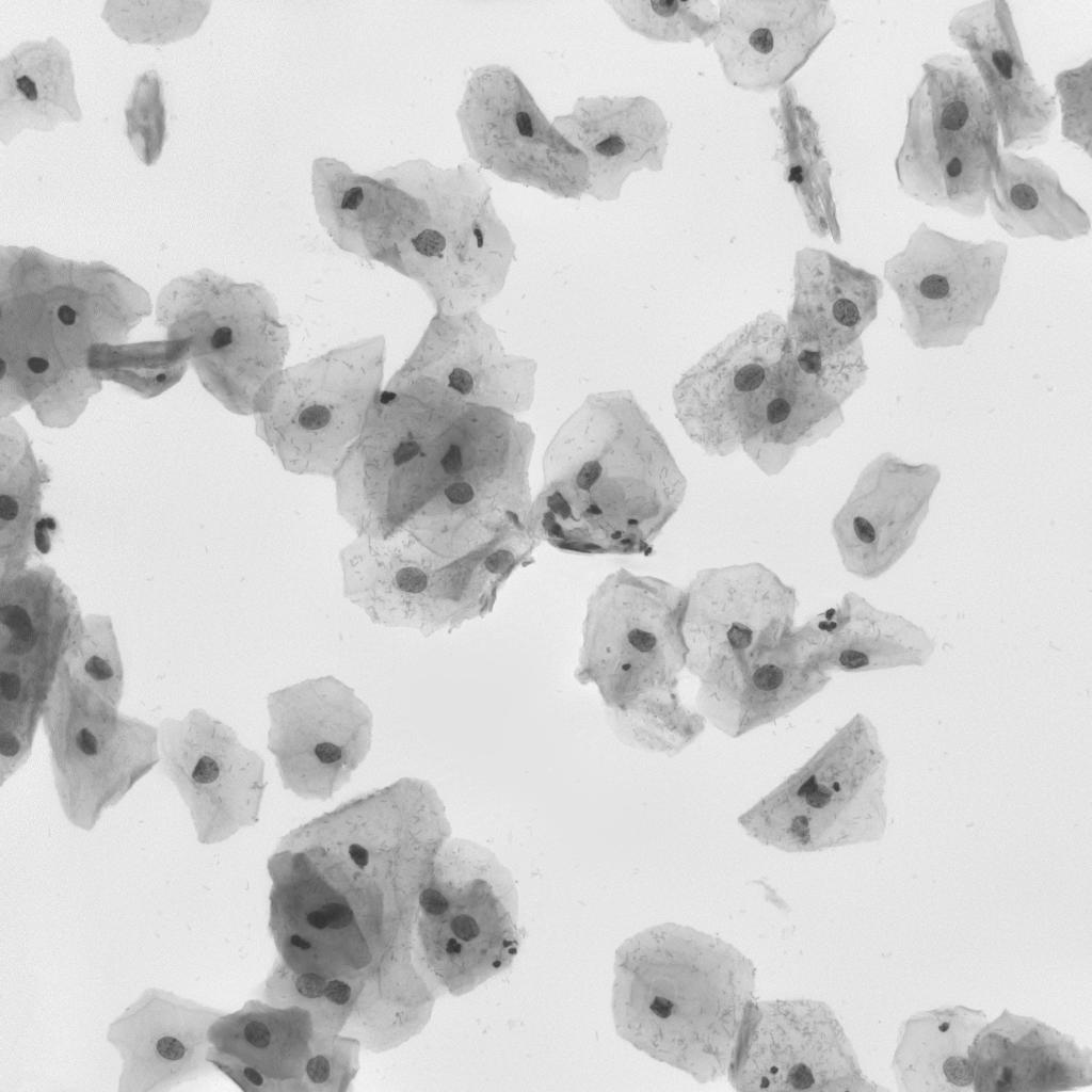 |
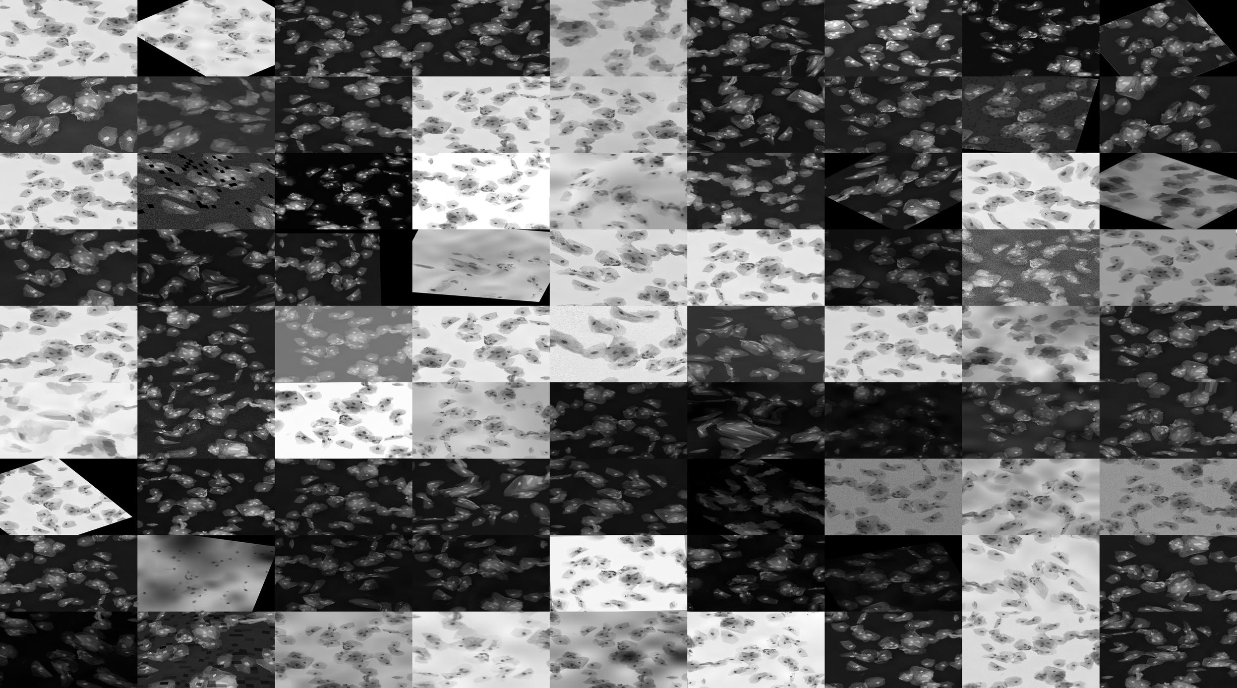 |
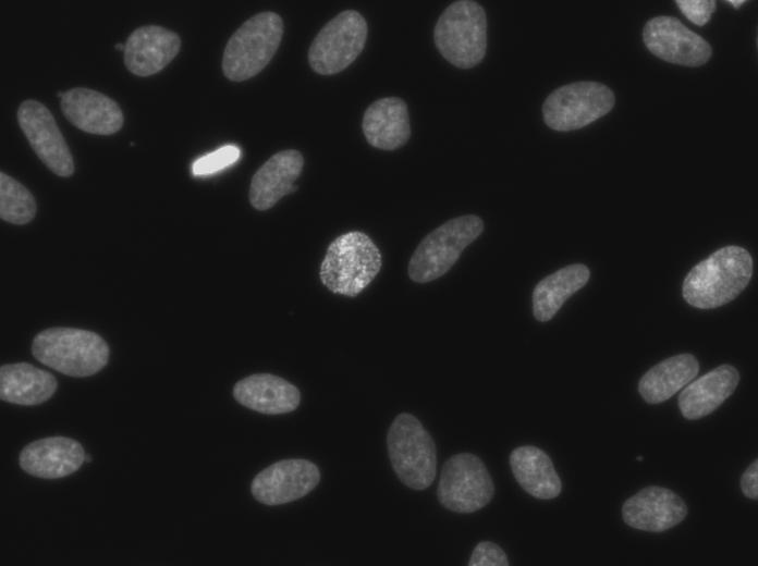 |
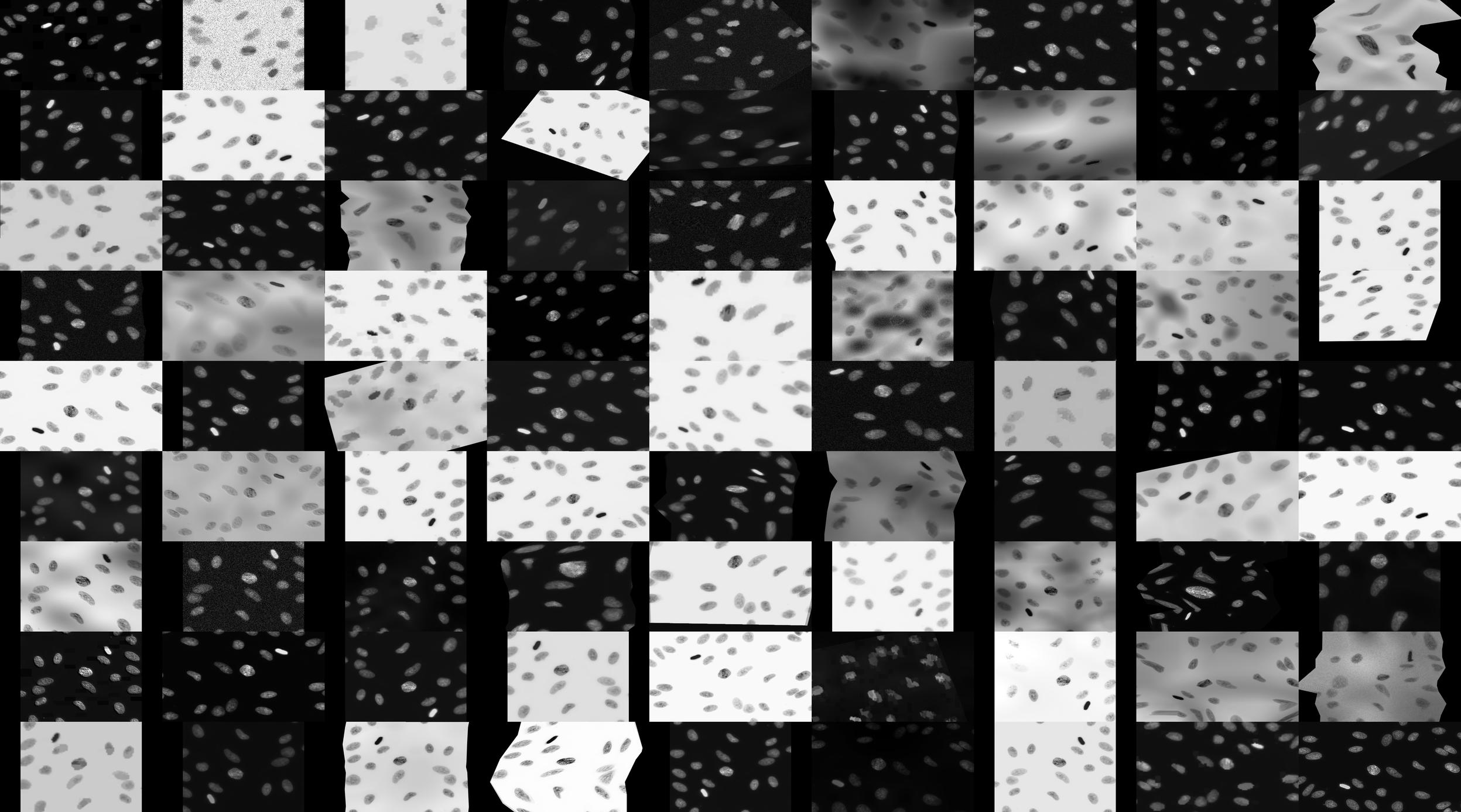 |
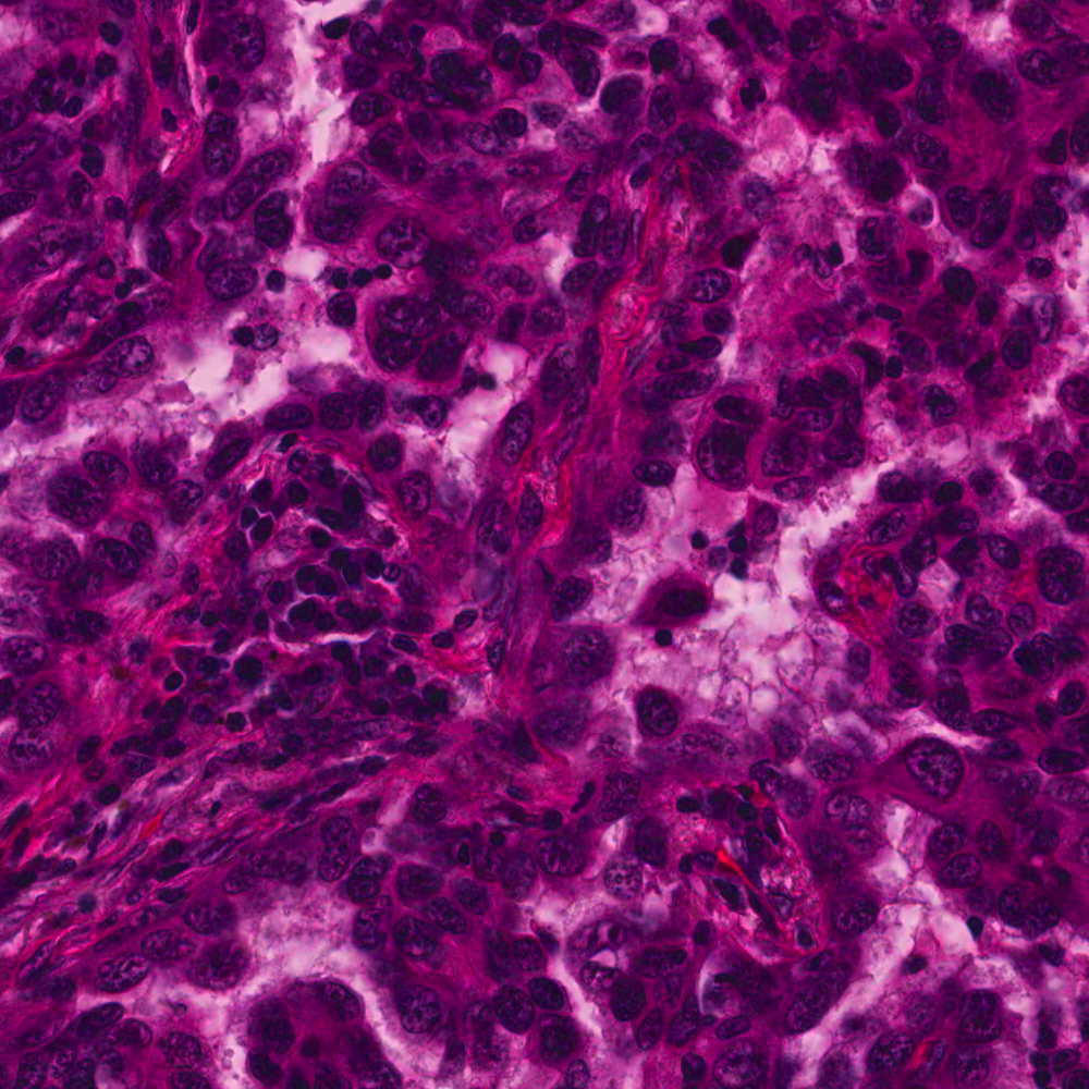
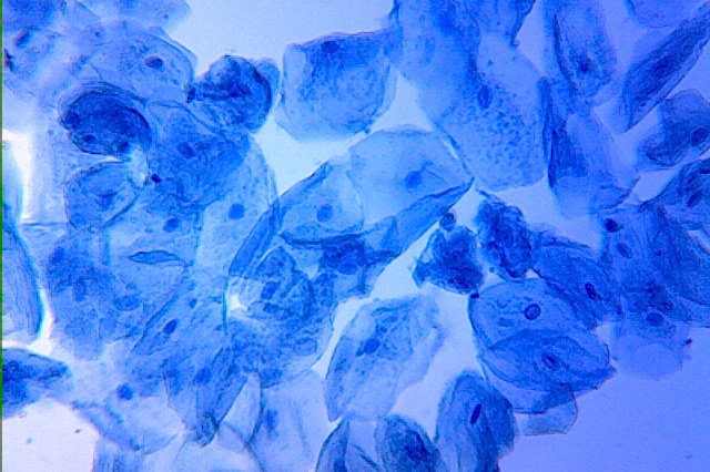
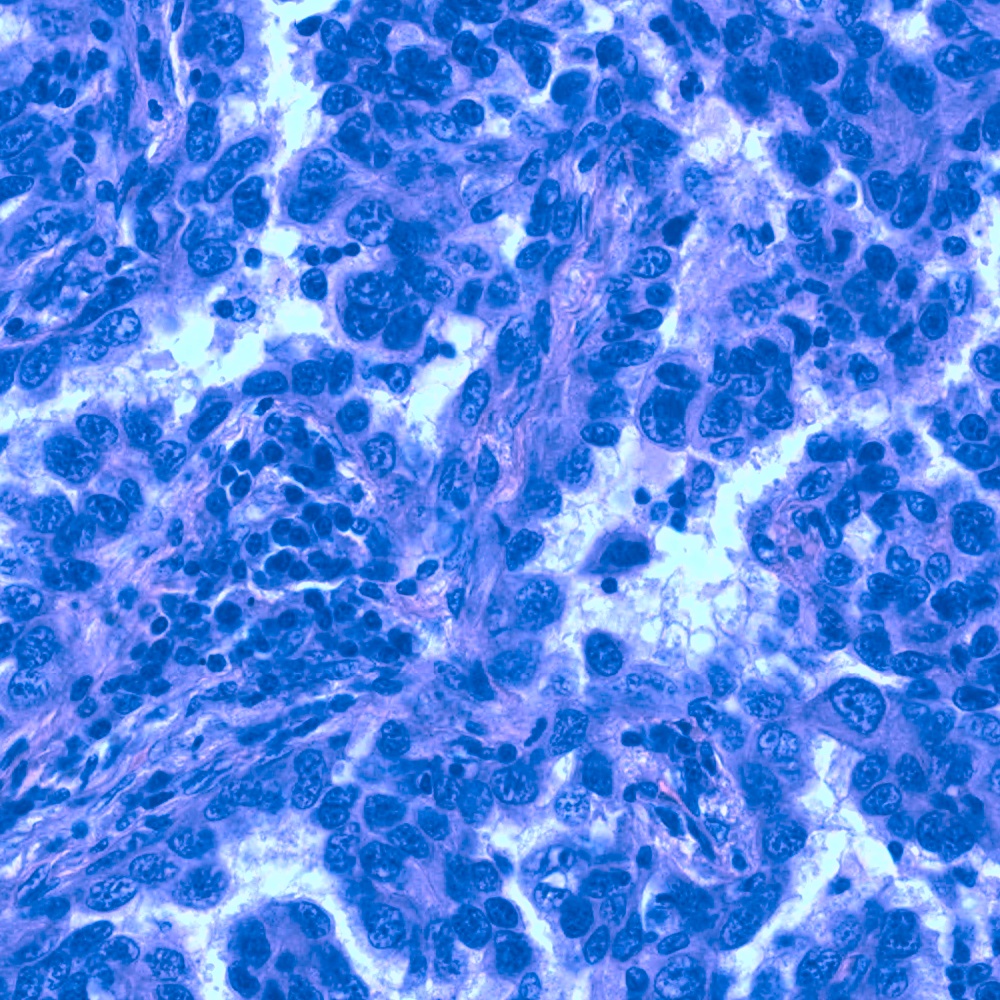
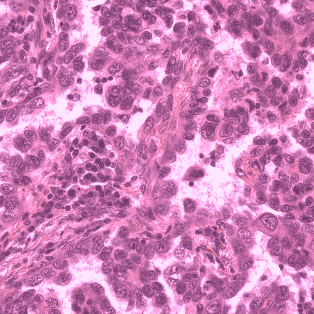
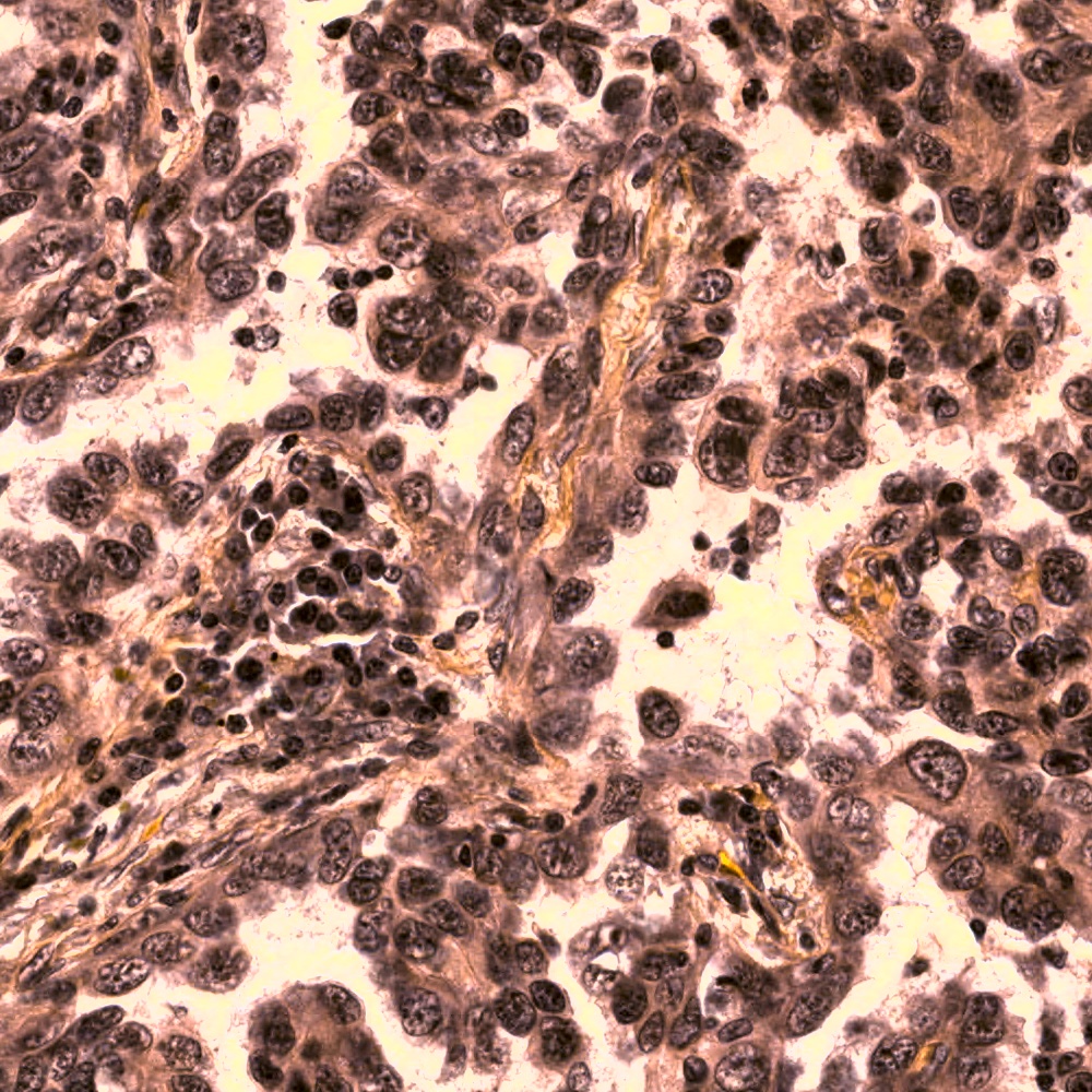
| Source Image | Target Image color style | Result Color Style |
|---|---|---|
 |
 |
 |
 |
 |
 |
 |
- Invert: Have improved the performance a lot
- Multiple Scales 900, 1000, 1100
- Flip left right
Detectron network configuration changes from the baseline e2e_mask_rcnn_X-152-32x8d-FPN-IN5k_1.44x.yaml are:
- Create small anchor sizes for small nuclei. RPN_ANCHOR_START_SIZE: 8 # default 32
- Add more aspect rations for nuclei that are close but in cylindrical structure. RPN_ASPECT_RATIOS: (0.2, 0.5, 1, 2, 5)
- Increase the ROI resolution. ROI_XFORM_RESOLUTION: 14
- Increase the number of detections per image from default 100. DETECTIONS_PER_IM: 500
- Decreased warmup fraction to 0.01
- Increased warmup iterations to 10,000
- Gave mask loss more weight WEIGHT_LOSS_MASK: 1.2
- Threshold on area to remove masks below area of 15 pixels
- Threshold on BBox confidence of 0.9
- Mask NMS
- On decreasing order of confidence, simple union-mask strategy to remove overlapping segments or cut segments at overlaps if overlap is below 30% of the mask.
- Inversion in augmentation
- Blurring and frequency noise
- Additional datasets, even though they caused a drop on the public leaderboard, I noticed no drop in local validation set.
- Mask dilations and erosions
- This did not have any improvement in the segmentation in my experiments
- Use contour approximations in place of original masks
- This did not have any improvement either. Maybe this could add a boost if using light augmentations.
- Randomly apply structuring like open-close
- Soft NMS thresh
- Did not improve accuracy
- Color images
- Did not perform as well as grey images after augmentations
- Color style transfer. Take a source image and apply the color style to target image.
- Style transfer: Was losing a lot of details on some nuclei but looked good on very few images.
- Dilation of masks in post processing, this drastically increased error because the model masks are already good.
- Distance transform and split masks during training.
- Ensemble multiple Mask R-CNN's
- Two stage predictions with U-Net after box proposals.
- Augmentation smoothing during training
- Increase the noise and augmentation slowly during the training phase, like from 10% to 50%
- Reduce the augmentation from 90% to 20% during training, for generalization and fitting.
- Experiment with different levels of augmentation individually across, noise, blur, texture, alpha blending.
- Different layer normalization techniques, with batch size more than one image at a time. Need bigger GPU.
- Little bit of hyperparameter search on thresholds and network architecture.
U-Net with watershed, did not think this approach would outperform Mask R-CNN
For basic host setup of Nvidia driver and Nvidia-Docker go to setup.sh.
Please find installation instructions for Caffe2 and Detectron in INSTALL.md.
chmod +x bin/nuclei/train.sh && ./bin/nuclei/train.sh -e 1_aug_gray_0_5_0 -v 1_aug_gray_0_5_0 -g 1 &

chmod +x bin/nuclei/test.sh && ./bin/nuclei/test.sh -e 1_aug_gray_1_5_1_stage_2_v1 -v 1_aug_gray_1_5_1_stage_2_v1 -g 1 &

tail -f /detectron/lib/datasets/data/logs/test_log

python lib/datasets/nuclei/write_submission.py \
    --results-root /detectron/lib/datasets/data/results/ \
    --run-version '1_aug_gray_1_5_1_stage_2_v1' \
    --iters '65999' \
    --area-thresh 15 \
    --acc-thresh 0.9 \
    --intersection-thresh 0.3
-
Detectron. Ross Girshick and Ilija Radosavovic. Georgia Gkioxari. Piotr Doll'{a}r. Kaiming He. Github, Jan. 2018.
-
Image augmentation for machine learning experiments. Alexander Jung. Github, Jan. 2015.
-
Normalizing brightfield, stained and fluorescence. Kevin Mader. Kaggle Notebook, Apr. 2018.
-
Fast, tested RLE and input routines. Sam Stainsby. Kaggle Notebook, Apr. 2018.
-
Example Metric Implementation. William Cukierski. Kaggle Notebook, Apr. 2018.
A collection of datasets converted into COCO segmentation format.
- Resized few images
- Tiled some images with lot of annotations to fit in memory
- Extracted masks when only outlines were available
- This is done by finding contours
DATASETS = {
    'nuclei_stage1_train': {
        IM_DIR:
            _DATA_DIR + '/Nuclei/stage_1_train',
        ANN_FN:
            _DATA_DIR + '/Nuclei/annotations/stage1_train.json'
    },
    'nuclei_stage_1_local_train_split': {
        IM_DIR:
            _DATA_DIR + '/Nuclei/stage_1_train',
        ANN_FN:
            _DATA_DIR + '/Nuclei/annotations/stage_1_local_train_split.json'
    },
    'nuclei_stage_1_local_val_split': {
        IM_DIR:
            _DATA_DIR + '/Nuclei/stage_1_train',
        ANN_FN:
            _DATA_DIR + '/Nuclei/annotations/stage_1_local_val_split.json'
    },
    'nuclei_stage_1_test': {
        IM_DIR:
            _DATA_DIR + '/Nuclei/stage_1_test',
        ANN_FN:
            _DATA_DIR + '/Nuclei/annotations/stage_1_test.json'
    },
    'nuclei_stage_2_test': {
        IM_DIR:
            _DATA_DIR + '/Nuclei/stage_2_test',
        ANN_FN:
            _DATA_DIR + '/Nuclei/annotations/stage_2_test.json'
    },
    'cluster_nuclei': {
        IM_DIR:
            _DATA_DIR + '/Nuclei/cluster_nuclei',
        ANN_FN:
            _DATA_DIR + '/Nuclei/annotations/cluster_nuclei.json'
    },
    'BBBC007': {
        IM_DIR:
            _DATA_DIR + '/Nuclei/BBBC007',
        ANN_FN:
            _DATA_DIR + '/Nuclei/annotations/BBBC007.json'
    },
    'BBBC006': {
        IM_DIR:
            _DATA_DIR + '/Nuclei/BBBC006',
        ANN_FN:
            _DATA_DIR + '/Nuclei/annotations/BBBC006.json'
    },
    'BBBC018': {
        IM_DIR:
            _DATA_DIR + '/Nuclei/BBBC018',
        ANN_FN:
            _DATA_DIR + '/Nuclei/annotations/BBBC018.json'
    },
    'BBBC020': {
        IM_DIR:
            _DATA_DIR + '/Nuclei/BBBC020',
        ANN_FN:
            _DATA_DIR + '/Nuclei/annotations/BBBC020.json'
    },
    'nucleisegmentationbenchmark': {
        IM_DIR:
            _DATA_DIR + '/Nuclei/nucleisegmentationbenchmark',
        ANN_FN:
            _DATA_DIR + '/Nuclei/annotations/nucleisegmentationbenchmark.json'
    },
    '2009_ISBI_2DNuclei': {
        IM_DIR:
            _DATA_DIR + '/Nuclei/2009_ISBI_2DNuclei',
        ANN_FN:
            _DATA_DIR + '/Nuclei/annotations/2009_ISBI_2DNuclei.json'
    },
    'nuclei_partial_annotations': {
        IM_DIR:
            _DATA_DIR + '/Nuclei/nuclei_partial_annotations',
        ANN_FN:
            _DATA_DIR + '/Nuclei/annotations/nuclei_partial_annotations.json'
    },
    'TNBC_NucleiSegmentation': {
        IM_DIR:
            _DATA_DIR + '/Nuclei/TNBC_NucleiSegmentation',
        ANN_FN:
            _DATA_DIR + '/Nuclei/annotations/TNBC_NucleiSegmentation.json'
    },
}import json
from pathlib import Path
import numpy as np
from PIL import Image
from pycocotools import mask as mask_util
ROOT_DIR = Path('/media/gangadhar/DataSSD1TB/ROOT_DATA_DIR/')
DATASET_WORKING_DIR = ROOT_DIR / 'Nuclei'
annotations_file = DATASET_WORKING_DIR / 'annotations/stage1_train.json'
COCO = json.load(open(annotations_file.as_posix()))
image_metadata = COCO['images'][0]
print image_metadata
# {u'file_name': u'4ca5081854df7bbcaa4934fcf34318f82733a0f8c05b942c2265eea75419d62f.jpg',
# u'height': 256,
# u'id': 0,
# u'nuclei_class': u'purple_purple_320_256_sparce',
# u'width': 320}
def get_masks(im_metadata):
image_annotations = []
for annotation in COCO['annotations']:
if annotation['image_id'] == im_metadata['id']:
image_annotations.append(annotation)
segments = [annotation['segmentation'] for annotation in image_annotations]
masks = mask_util.decode(segments)
return masks
masks = get_masks(image_metadata)
print masks.shape
# (256, 320, 37)
def show(i):
i = np.asarray(i, np.float)
m,M = i.min(), i.max()
I = np.asarray((i - m) / (M - m + 0.000001) * 255, np.uint8)
Image.fromarray(I).show()
show(np.sum(masks, -1))
# this should show an image with all masks-
2018 Data Science Bowl: Find the nuclei in divergent images to advance medical discovery. Competition, Kaggle, Apr. 2018. Download: https://www.kaggle.com/c/data-science-bowl-2018/data
-
2018 Data Science Bowl: Kaggle Data Science Bowl 2018 dataset fixes. Konstantin Lopuhin, Apr. 2018. Download: https://github.com/lopuhin/kaggle-dsbowl-2018-dataset-fixes
-
TNBC_NucleiSegmentation: A dataset for nuclei segmentation based on Breast Cancer patients. Naylor Peter Jack; Walter Thomas; Laé Marick; Reyal Fabien. 2018. Download: https://zenodo.org/record/1175282/files/TNBC_NucleiSegmentation.zip
-
A Dataset and a Technique for Generalized Nuclear Segmentation for Computational Pathology. Kumar N, Verma R, Sharma S, Bhargava S, Vahadane A, Sethi A. 2017. Download: https://nucleisegmentationbenchmark.weebly.com/dataset.html
-
Deep learning for digital pathology image analysis: A comprehensive tutorial with selected use cases. Andrew Janowczyk, Anant Madabhushi. 2016. Download: http://andrewjanowczyk.com/wp-static/nuclei.tgz
-
Nuclei Dataset: Include 52 images of 200x200 pixels. Jie Shu, Guoping Qiu, Mohammad Ilyas. Immunohistochemistry (IHC) Image Analysis Toolbox, Jan. 2015. Download: https://www.dropbox.com/s/9knzkp9g9xt6ipb/cluster%20nuclei.zip?dl=0
-
BBBC006v1: image set available from the Broad Bioimage Benchmark Collection. Vebjorn Ljosa, Katherine L Sokolnicki & Anne E Carpenter. 2012. Download: https://data.broadinstitute.org/bbbc/BBBC007/
-
BBBC007v1: image set available from the Broad Bioimage Benchmark Collection. Vebjorn Ljosa, Katherine L Sokolnicki & Anne E Carpenter. 2012. Download: https://data.broadinstitute.org/bbbc/BBBC006/
-
BBBC018v1: image set available from the Broad Bioimage Benchmark Collection. Vebjorn Ljosa, Katherine L Sokolnicki & Anne E Carpenter. 2012. Download: https://data.broadinstitute.org/bbbc/BBBC018/
-
BBBC020v1: image set available from the Broad Bioimage Benchmark Collection. Vebjorn Ljosa, Katherine L Sokolnicki & Anne E Carpenter. 2012. Download: https://data.broadinstitute.org/bbbc/BBBC020/
-
Nuclei Segmentation In Microscope Cell Images: A Hand-Segmented Dataset And Comparison Of Algorithms. L. P. Coelho, A. Shariff, and R. F. Murphy. Proceedings of the 2009 IEEE International Symposium on Biomedical Imaging (ISBI 2009), pp. 518-521, 2009. Download: http://murphylab.web.cmu.edu/data/2009_ISBI_2DNuclei_code_data.tgz
