Roberock / Stochastic-area-metric

Code for computing the stochastic area metric in Python and Matlab.

Area metric code

This repository gathers code for computing the stochastic area metric, in Python.

To cite this repository use:

De Angelis M., Sunny J. (2021). Stochastic area metric. Github repository.

https://github.com/marcodeangelis/Stochastic-area-metric/

doi: https://doi.org/10.5281/zenodo.4419644

or the BibTex:

@misc{DS2021,
  author = {De Angelis, M., Sunny, J.},
  title = {Stochastic area metric},
  year = {2021},
  publisher = {GitHub},
  journal = {GitHub repository},
  doi = {10.5281/zenodo.4419645},
}

For more about the stochastic area distance or Wasserstein distance the reader is referred to the following references:

[1] https://en.wikipedia.org/wiki/Wasserstein_metric

[2] Ramdas, Garcia, Cuturi “On Wasserstein Two Sample Testing and Related Families of Nonparametric Tests” (2015). arXiv:1509.02237. https://arxiv.org/pdf/1509.02237.pdf

Disclaimer: This code library has been developed for research, testing, and educational reasons. It is by no means optimized to deal with large datasets. With large datasets we reccommed the use of the scipy package. An optimized version of this library is currently under development.

Get started

Clone the repository using:

$ git clone [e-mail]:marcodeangelis/stochastic-area-metric.git

On MacOS/Linux:

$ python3 -m venv venv 

$ source venv/bin/activate

(venv) $ pip install -r requirements.txt

On Windows10:

$ python -m venv venv

$ venv\Scripts\activate

(venv) $ pip install -r requirements.txt

Let's import the Python module for the area metric

import areametric as am

We can use the dot notation to access:

• The class Dataset
• The function areaMe
• The function plot
• The class ParametricDataset

This is all we are going to need to demonstrate the use of the code library in this repository.

Datasets of the same size

Let's create two datasets with the same number of elements

Notice:

The datasets need to be created as Python lists and not as numpy arrays.

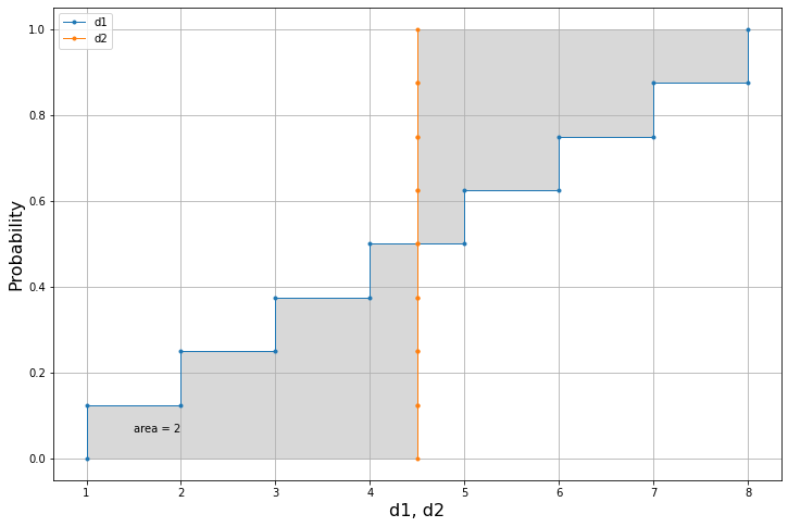
d1 = [1,2,3,4,5,6,7,8]
d2 = [4.5]*8

We can already use the code to compute the area metric in just one line:

print(am.areaMe(d1,d2))

2.0

We can then use the plot function to visualise the results in a single plot.

am.plot(d1,d2)

Let's consider two different datasets.

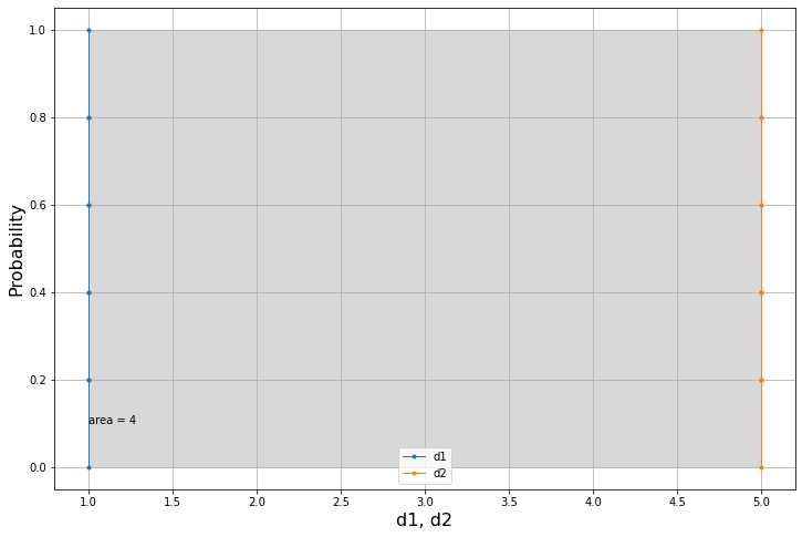
d1=5*[1.]
d2=5*[5.]

We would expect this difference to be equal to 4.0 as these two datasets are equvalent to two points.

am.areaMe(d1,d2)

4.0

The plot confirms this intuition.

am.plot(d1,d2)

The Dataset class

We can make use of the Dataset class in several ways. One of these is to obtain the same results with some syntactic sugar, so in a more elegant way.

d1,d2 = [1,2,3,4,5,6,7,8],[4.5]*8
D1 = am.Dataset(d1)
D2 = am.Dataset(d2)

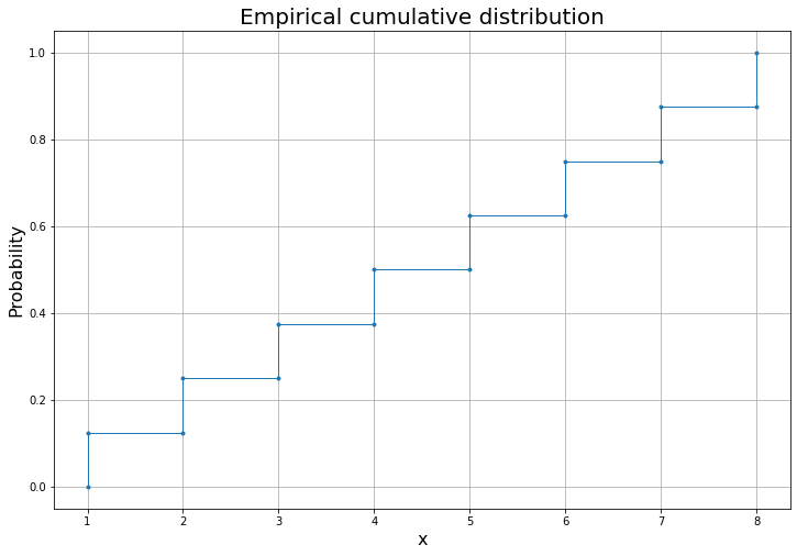
We can plot the individual datasets:

D1.plot()

And we can compute the area metric using the subtraction operator -.

D1-D2

2.0

The infix operator - that implements the area-metric is commutative as we expected because it is in all respects a true metric. So swapping the operands will yield the same answer.

D2-D1

2.0

Datasets of different size

This category of datasets will come soon.

Parametric datasets

Parametric datasets are datasets obtained from parametric distributional models such as the Lognormal distribution.

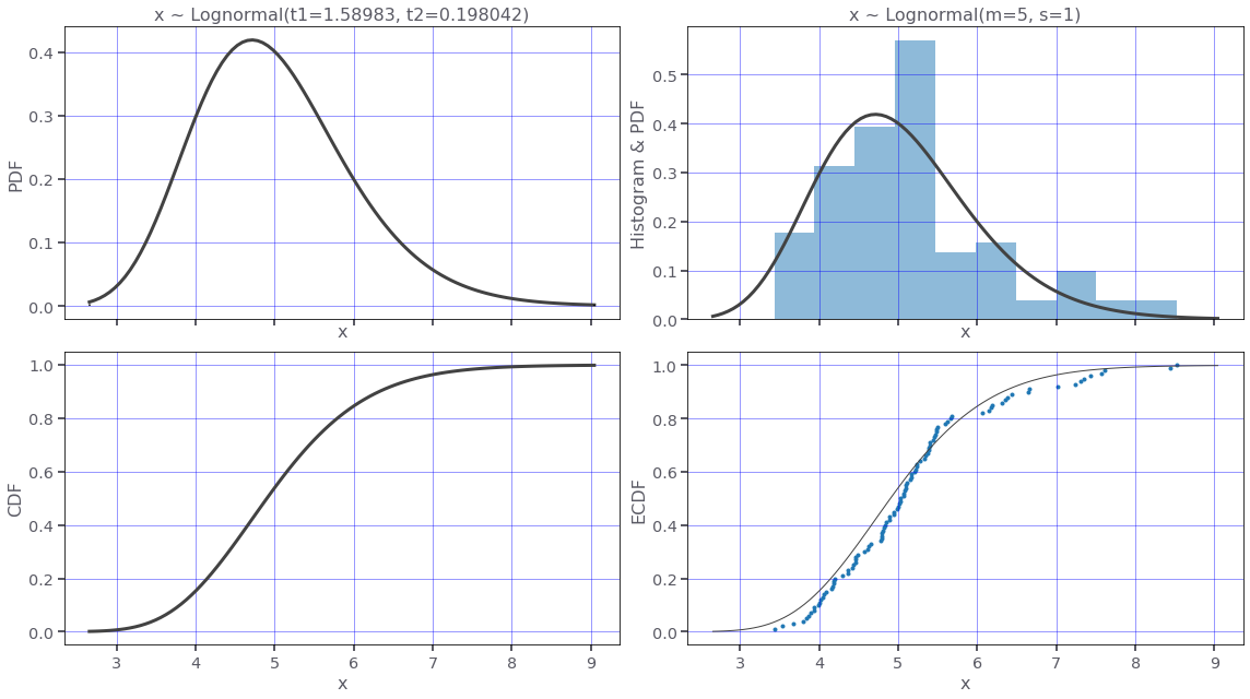
Let's define a Lognormal distribution using the moments.

lognormal_dist = am.Lognormal(5,1)
print(lognormal_dist)

x ~ Lognormal(m=5, s=1)

Let's plot this distribution.

lognormal_dist.plot(N=100)

Now we can use the Lognormal distribution to generate two datasets.

We will use different mean and standard-deviation for the two datasets.

lognormal_dist_1 = am.Lognormal(5,1)
lognormal_dist_2 = am.Lognormal(7,4)

We can now generate the datasets using the method sample.

We will generate a big number of samples to test the speed of the code.

d1 = am.Dataset(list(lognormal_dist_1.sample(N=100_000)))
d2 = am.Dataset(list(lognormal_dist_2.sample(N=100_000)))

d1-d2

2.319762595668186

Below we time the execution. It takes a small fraction of a second (0.265 s) to compute the distance between two datasets with 1e5 elements.

%timeit d1-d2

265 ms ± 3.95 ms per loop (mean ± std. dev. of 7 runs, 1 loop each)

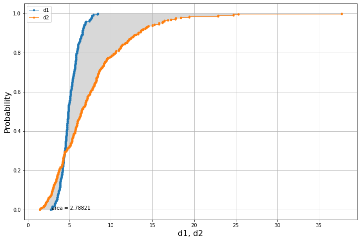
The plot is done using less samples as accuracy is not a priority.

am.plot(list(lognormal_dist_1.sample(N=300)),list(lognormal_dist_2.sample(N=300)))

The median difference is:

abs(lognormal_dist_1.median() - lognormal_dist_2.median())

1.1747986164166138

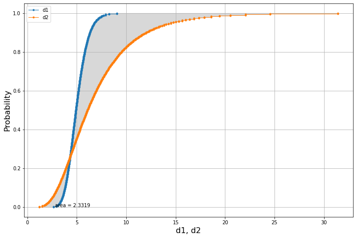
To get better accuracy we can generate the datasets using directly the inverse cumulative distribution, aka percent point function ppf. In this way we'll get rid of the sampling error, and we'll get an answer that is deterministic and not as sensitive to the cardinality of the dataset.

We'll use the class ParametricDataset to generate the data.

x1 = am.ParametricDataset(lognormal_dist_1, N=300)
x2 = am.ParametricDataset(lognormal_dist_2, N=300)
am.plot(x1.to_list(),x2.to_list())

x1-x2

2.3319029880776765

We can check that the obtained result coincides exactly with the result using the scipy code library, which is a very good news.

from scipy.stats import wasserstein_distance # https://docs.scipy.org/doc/scipy/reference/generated/scipy.stats.wasserstein_distance.html
wasserstein_distance(x1,x2)

2.331902988077677