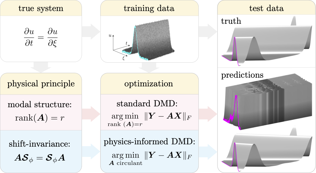
This repository contains codes that calculate physics-informed dynamic mode decompositions from data [1].
The dynamic mode decomposition [2] is a data-driven method that
- reduces high-dimensional data to a few coherent spatio-temporal patterns, and,
- identifies the linear operator that best represents the data.
Previous works have sought linear operators that are low rank. While this approach has seen enormous success, it is well known that classical DMD models are highly sensitive to noise, prone to overfitting, and do not respect known physical laws. Our recent paper [1] partially addresses these issues by incorporating prior known physics into the DMD procedure. Specifically, we rephrase the DMD optimization problem as
where X and Y are data matrices, A is a matrix and M is a matrix manifold. The matrix manifold is specified by the user and should be chosen based on prior physical knowledge of the system. Since the learned model, A, is restricted to lie on the selected matrix manifold, it necessarily obeys the required physical principles. The optimization problem (1) is known as a Procrustes problem. The codes herein solve (1) for a range of matrix manifolds; an example with a shift-invariant system is illustrated below:
The script pidmd.m solves the optimization problem (1) for a wide range of matrix manifolds.
For example, if we know that the system we are studying preserves the 2-norm (i.e. energy) of states, then we can restrict our model search to orthogonal matrices.
This is implemented by
model = piDMD(X, Y, 'orthogonal')The learned model is the best such linear model; it is a solution to (1).
Here, model is a function handle that takes vectors v as inputs and outputs the vector matrix product A*v where A is the learned orthogonal model.
The reason for this design choice is that the learned A is often so large that we cannot store it explicitly in memory.
If the model is desired explicitly then it can be formed by model(eye(n)), where n is the state dimension.
Further, the eigenvalues and eigenvectors of the model can be computed by, for example,
[model, eVals, eVecs] = piDMD(X, Y, 'orthogonal')This method exploits the structure of the matrix manifold to efficiently compute the model's eigendecomposition. As such, this technique is usually far more efficient than forming the model explicitly and computing the eigendecomposition.
See the `examples' folder for codes that reproduce the results in [1] as well as additional examples.
Here are the matrix manifolds currently implemented in this repository.
The last column refers to the argument passed in piDMD(X, Y, 'manifold').
| physics | matrix manifold | manifold |
|---|---|---|
| modal | low-rank | exact or exactSVDS |
| conservative | orthogonal (unitary) | orthogonal |
| Hermitian/anti-Hermitian | symmetric/skew-symmetric | symmetric or skewsymmetric |
| local | diagonal or banded | diagonal, diagonaltls, diagonalpinv |
| local and Hermitian (self-adjoint) | symmetric and tridiagonal | symtridiagonal |
| causal/anti-causal | upper/lower triangular | uppertriangular or lowertriangular |
| shift-invariant and periodic (1D) | circulant | circulant or circulantTLS |
| shift-invariant and periodic (1D) and conservative/Hermitian/anti-Hermitian | circulant and unitary/symmetric/skew-symmetric | circulantunitary / circulantsymmetric / circulantskewsymmetric |
| shift-invariant and periodic (2D) | block-circulant-circulant-block (BCCB) | BCCB or BCCBtls |
| shift-invariant and periodic (2D) and conservative/Hermitian/anti-Hermitian | BCCB and unitary / symmetric / skew-symmetric | BCCBunitary / BCCBsymmetric / BCCBskewsymmetric |
| shift-invariant/anti-shift-invariant (1D) | Toeplitz/Hankel | toeplitz / hankel |
The suffix tls indicates that the problem is solved in the total least squares sense.
If your matrix manifold is not currently included in this software then Manopt may be able to help. There is an example of using Manopt to solve the Procrustes problem here.
To start using piDMD, simply clone this repository to your MATLAB directory.
The codes are written in MATLAB and were tested in MATLAB 2021b on a 2021 Macbook Pro with Apple M1 chip, 8 cores and 16 GB of RAM. Each example should take a couple of seconds to run.
[1] Physics-informed dynamic mode decomposition (piDMD)
Peter J. Baddoo, Benjamin Herrmann, Beverley J. McKeon, Nathan J. Kutz & Steven L. Brunton, arXiv:2112.04307
[2] Dynamic mode decomposition of numerical and experimental data
Peter J. Schmid, J. Fluid Mech., vol. 656, pp. 5–28, 2010.

