bavDiv - Species richness changes in Bavaria, Germany: Differences between protected and non-protected areas
Table 1. Model performance (BIC) of different variable combinations for each taxon (Aves, Lepidoptera, Odonata, Orthoptera) and all taxa together (Total).
| formula | Aves | Lepidoptera | Odonata | Orthoptera | Total |
|---|---|---|---|---|---|
| sum_art ~ s(jahr) + s(sum_n) | 146364.8 | 252721.6 | 61695.34 | 64640.47 | 487483.4 |
| sum_art ~ s(jahr) + s(XLU) + s(YLU) + s(sum_n) | 145439.5 | 249448.7 | 61483.04 | 64149.92 | 481724.3 |
| sum_art ~ s(jahr) + s(XLU, YLU) + s(sum_n) | 145159.7 | 244228.6 | 61459.43 | 64102.48 | 475467.1 |
| sum_art ~ mon + s(jahr) + s(sum_n) | 129356.8 | 312108.6 | 79512.01 | 77502.65 | 717109.9 |
| sum_art ~ mon + s(jahr) + s(XLU) + s(YLU) + s(sum_n) | 128904.3 | 308684.6 | 79460.11 | 77311.58 | 713027.6 |
| sum_art ~ mon + s(jahr) + s(XLU, YLU) + s(sum_n) | 128880.9 | 304120.0 | 79451.93 | 77313.70 | 706953.7 |
Table 2. Model variance (R2) of different variable combinations for each taxon (Aves, Lepidoptera, Odonata, Orthoptera) and all taxa together (Total).
| formula | Aves | Lepidoptera | Odonata | Orthoptera | Total |
|---|---|---|---|---|---|
| sum_art ~ s(jahr) + s(sum_n) | 0.765 | 0.704 | 0.716 | 0.679 | 0.659 |
| sum_art ~ s(jahr) + s(XLU) + s(YLU) + s(sum_n) | 0.768 | 0.714 | 0.724 | 0.696 | 0.665 |
| sum_art ~ s(jahr) + s(XLU, YLU) + s(sum_n) | 0.770 | 0.733 | 0.726 | 0.701 | 0.681 |
| sum_art ~ mon + s(jahr) + s(sum_n) | 0.744 | 0.698 | 0.751 | 0.738 | 0.588 |
| sum_art ~ mon + s(jahr) + s(XLU) + s(YLU) + s(sum_n) | 0.752 | 0.716 | 0.757 | 0.747 | 0.604 |
| sum_art ~ mon + s(jahr) + s(XLU, YLU) + s(sum_n) | 0.752 | 0.735 | 0.760 | 0.750 | 0.625 |
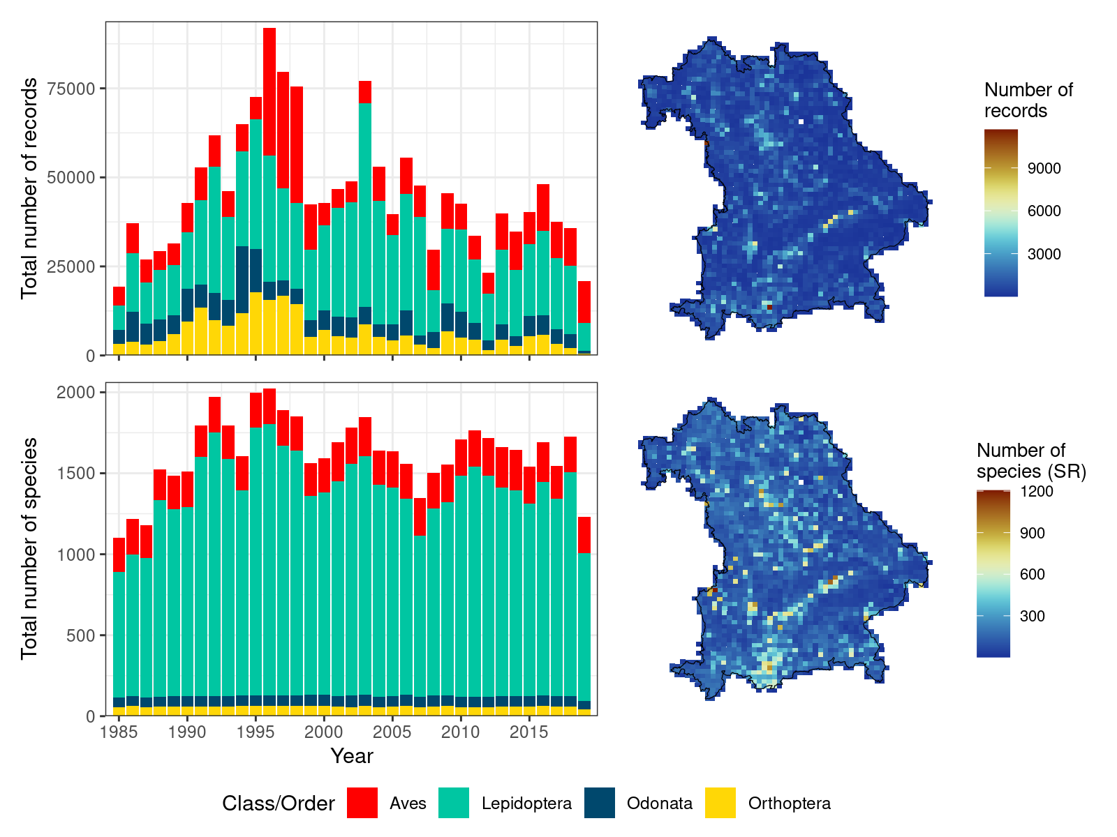
Figure 1. a) Number of observations recorded per year, b) number of observations per grid cell, c) Species richness recorded per year, d) Species richness per grid cell. Different colours represent number of species per taxonomic group.
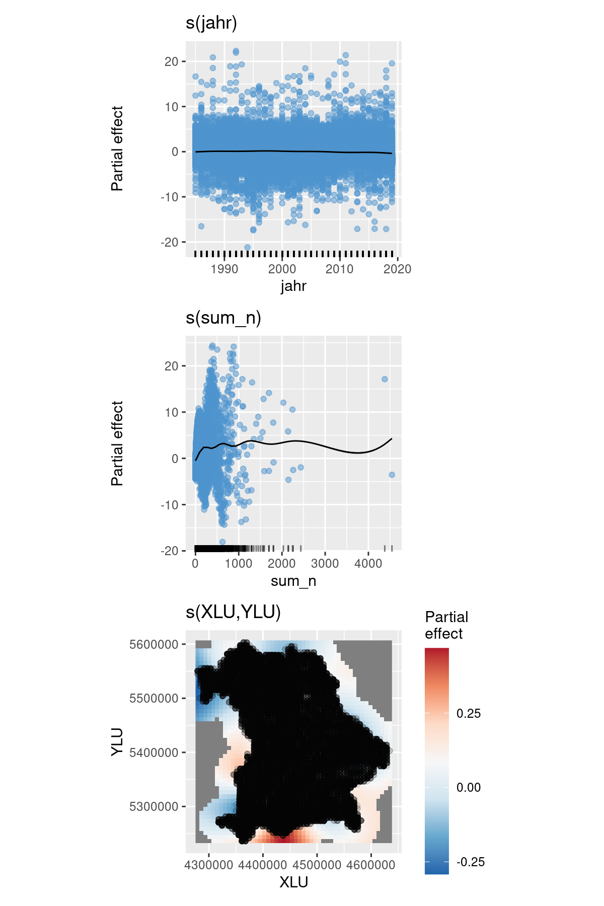
Figure 2. Generalized additive model (GAM) plots showing the partial effects on total species richness. Tick marks on the x-axis are observed data points. The y-axis represents the effect function of isolation on Kipp’s distance. Dark gray shadows indicate 95% confidence bounds. (Note that the scale of the y-axis differs between the two columns).
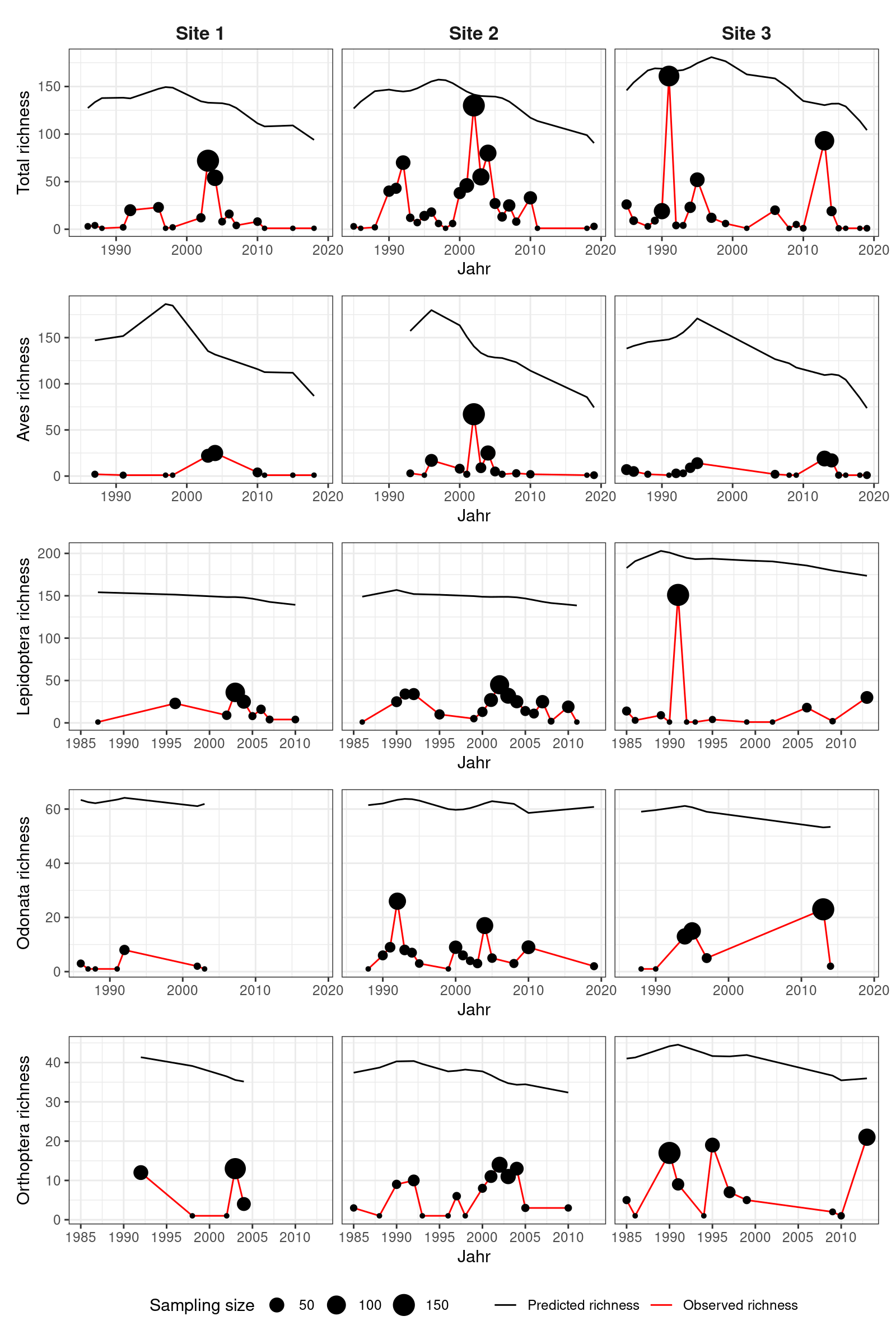
Figure 3. Observed and modeled species richness over time for three randomly selected sites. Modeled species richness was predicted for a sampling effort of N = 500.
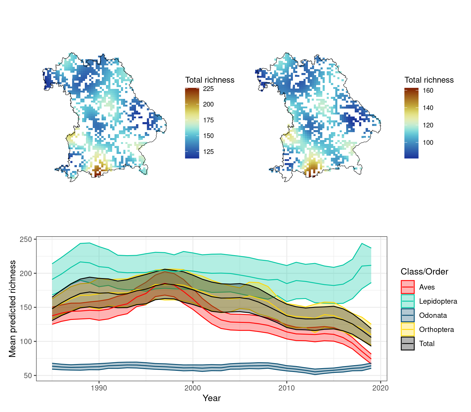
Figure 4. a) past (1985) and b) present (2018) modeled species richness, as well as the mean modeled species richness over time for Bavaria. Modeled species richness was predicted for a sampling effort of N = 500.
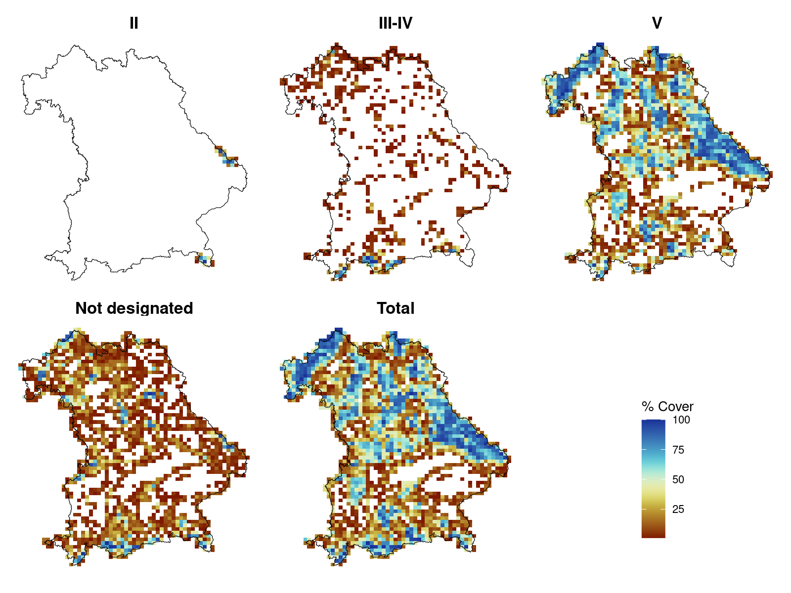
Figure 5. Map of percentage cover per grid cell for the different IUCN protection categories.
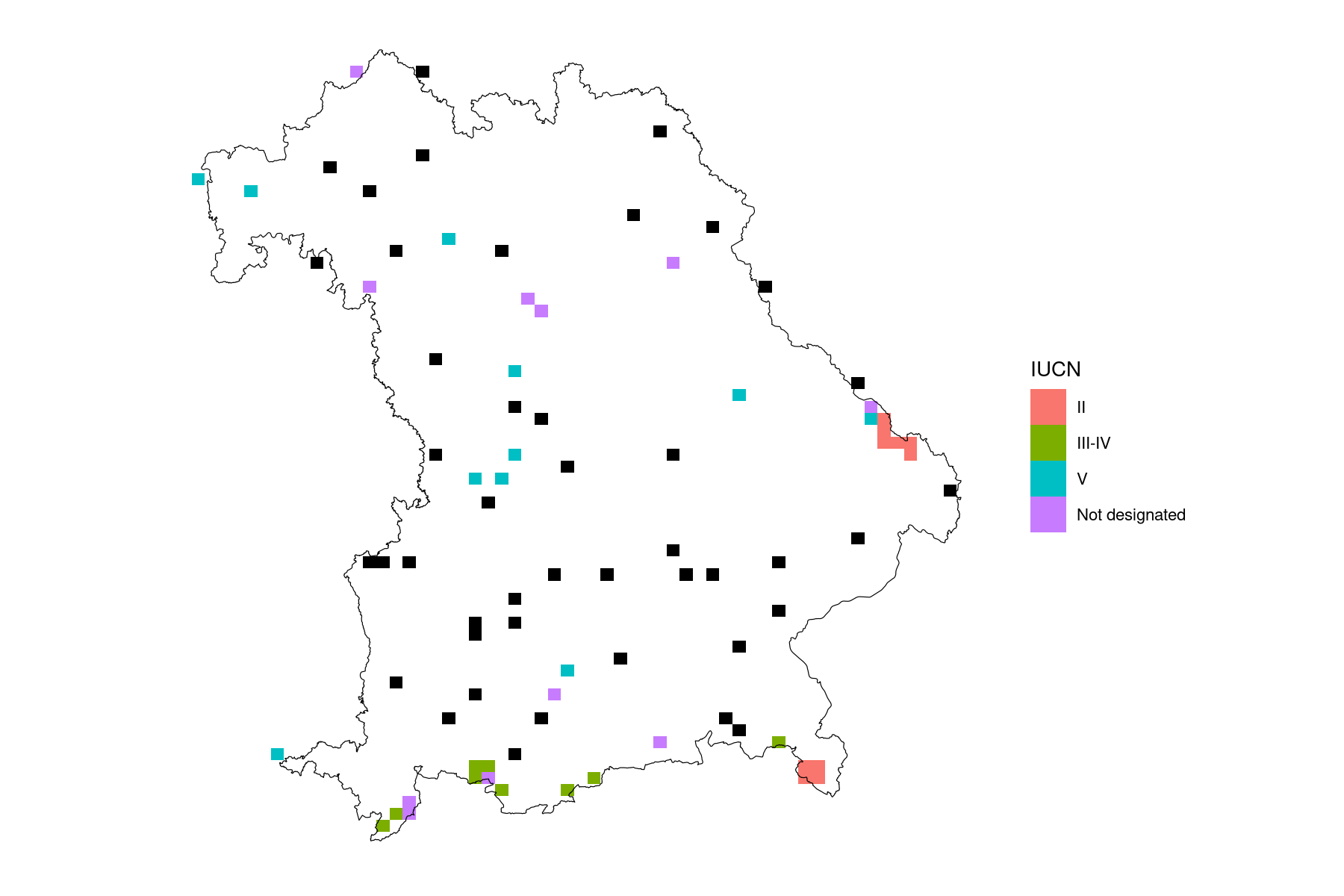
Figure 6. Randomly sampled locations with sufficient observations (N >= 20) for non-protected grid cells (Protection < 20 %, N = 68, black) and protected grid cells (Protection >= 20 %, N = 68) for each IUCN category present (II, III-V, V and Not-Reported, N = 17).
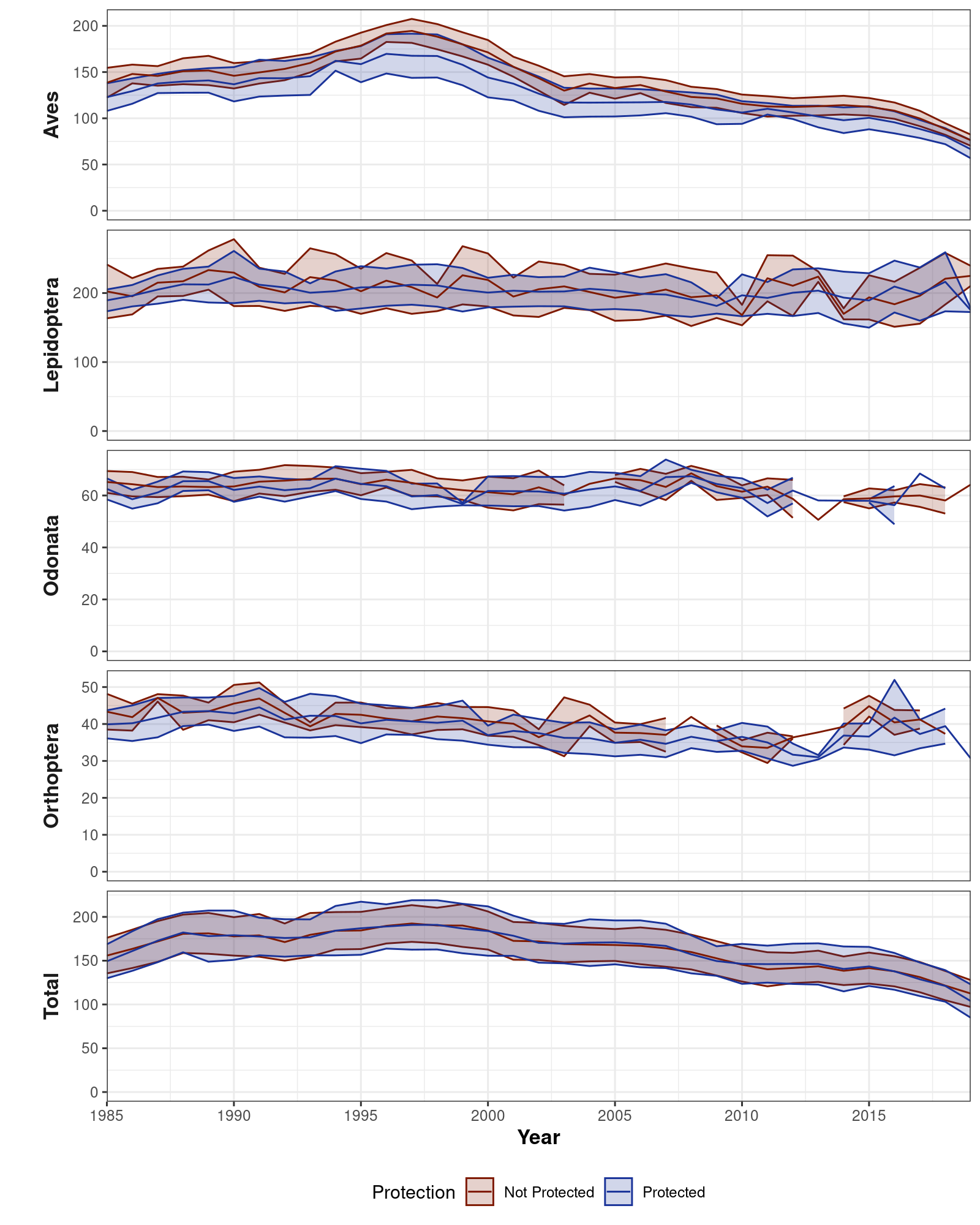
Figure 7. Plot of species richness over time separately for each taxonomic group and for protected versus non-protected areas.
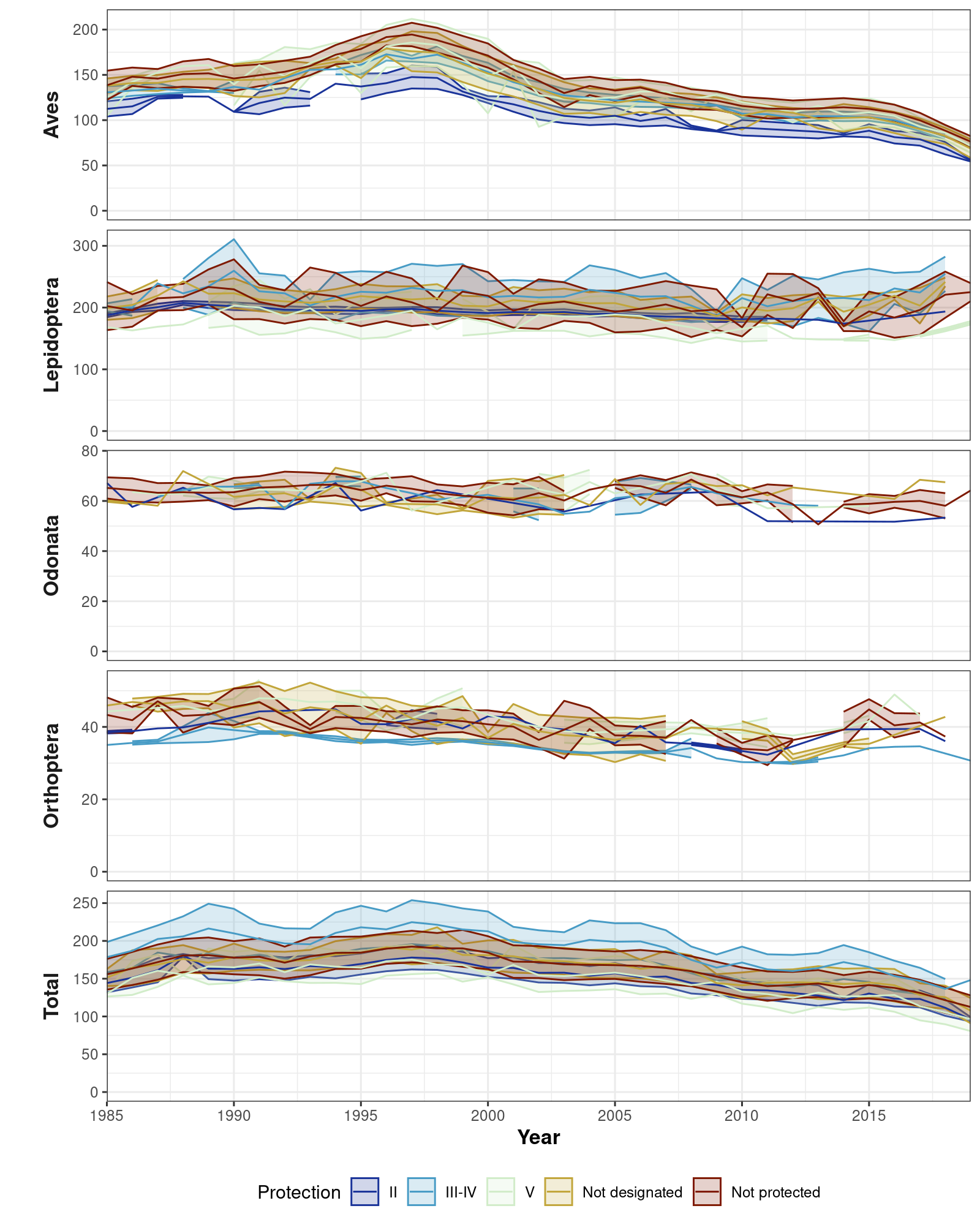
Figure 8. Plot of species richness, sampling effort and species richness/sampling effort over time for protected areas divided into the different IUCN categories.
