RRRChangeche / Stanford-cs131-2020

My solution of Stanford Computer Vision Foundations and Applications CS131 (Fall 2020) assignments.

CS131: Computer Vision Foundations and Applications

Course link

This repository contains the released assignment for the fall 2020 of CS131, a course at Stanford taught by Juan Carlos Niebles and Ranjay Krishna.

Assignments

• Environment: python3.6+
• Requirements: run "pip install -r requirements.txt"

Outline

• hw0 - Basics
• hw1 - Filters
• hw2 - Edges detect - Smart car lane detection
• hw3 - Panorama - Image stitching
• hw4 - Segmentation - clustering
• hw5 - Seam carving
• hw6 - Object detection
• hw7 - Tracking - optical flow
• hw8 - Camera Models

hw0 - Basics [link]

• Linear Algebra and Numpy review
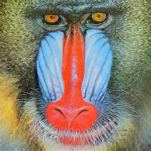
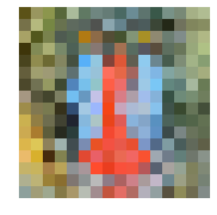
• Image manipulation
  • laod image
  • crop image
  • image dimmer
  • resize image
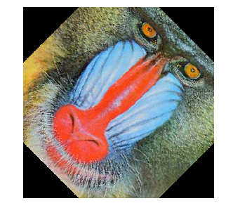
  • Rotating 2D coordinates
  • Rotate image

load image	blur	rotate

hw1 - Filters [link]

(Lecture 03)

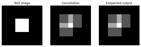
• Convolution

  • prove Commutative property
  • prove Shift invariance
  • prove Linearity
  • Implementation
    • conv_nested - using 4 for-loops
    • conv_fast - using zero-pad and numpy dot product
      1. zero padding
      2. flip kernel vertically and horizontally
      3. compute weighted sum

• Cross-correlation

  • Template matching
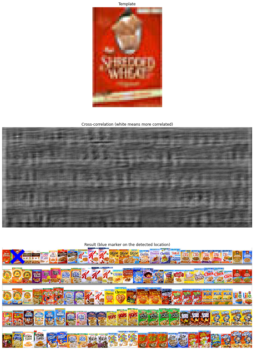
  • Zero-mean cross-correlation
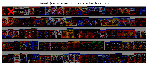
  • Normalized cross-correlation

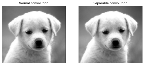
• Separable Filter

  • Theory
  • Complexity comparison

What did I learn?

• Optimize convolution implementaion by using numpy(conv_fast).

• It's about up to 15x faster than naive implementation(conv_nested) in this case.

• The Zero-mean Cross-Correlation is not robust to change in lighting condition.

• Implement template matching by Normalized Cross-Correlation algorithm to search the target pattern in the source image.

• 2D separable convolution is equivalent to two 1D convolutions.

• Optimize 2D convolution by doing two 1D convolutoins.

• It's about 2x faster by using separable filter in this case.

Pictures
Convolution
Zero-mean cross-correlation
Normalized cross-correlation
Normal V.S. Separable convolution

Recitation 4 - Advanced Numpy Tutorial: [link]

• Creating numpy array
• Array Attributes
• Accessing elements
• Matrix operations
  • Element-wise operation - all arithmetic operations are applied to a matrix element-wise
    • +, -, *, /
    • sqrt/ power
  • Axis-based operations
    • mean
    • std
    • sum
  • Some other useful manipulations
    • concatenate
    • tranpose
    • linalg.inv - to invert a matrix
• Numpy for linear algebra
  • Dot product - np.dot - return scalar
  • np.matmul/ @
• Numpy arrays, references, and copies
  • import copy/ copy.copy() and copy.deepcopy()
  • np.array.copy()
• Sorting
  • np.sort - return sorted array
  • np.argsort - return sorted indices
• Reshaping
• Broadcsting
• Using boolean masks
  • boolean masks
  • np.where
• Linear Algebra
  • np.linalg.slove
  • np.linalg.lstsq
  • $\theta = (X^T X)^{-1} X^T y$
• Vectorize equations

What did I learn?

• All arithmetic operations are applied to a matrix element-wise.

• Numpy operation is way faster than list.

• Reference of numpy array, point to the same object. Use copy to fix this.

• Be aware of copy and deepcopy.

• Broadcasting - Two dimensions are compatible when they are equal, or one of them is 1. (details) ex: c = a*b, when a's shape is (1,3)/ b's shape is (3,1), then c's shape is (3,3) because of broadcasting operation.

hw2 - Edges detect - Smart car lane detection [link]

(Lecture 03-04)

• Canny edge detector
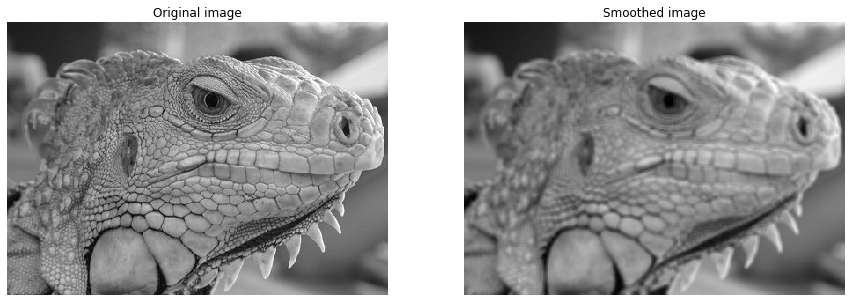
  1. Smoothing
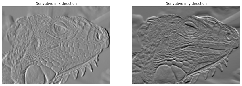
  2. Finding gradients
  3. Non-maximum suppression
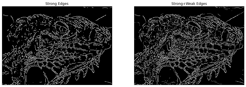
  4. Double thresholding
  5. Edge tracking by hysterisis
  6. Optimize parameters
• Lane detection
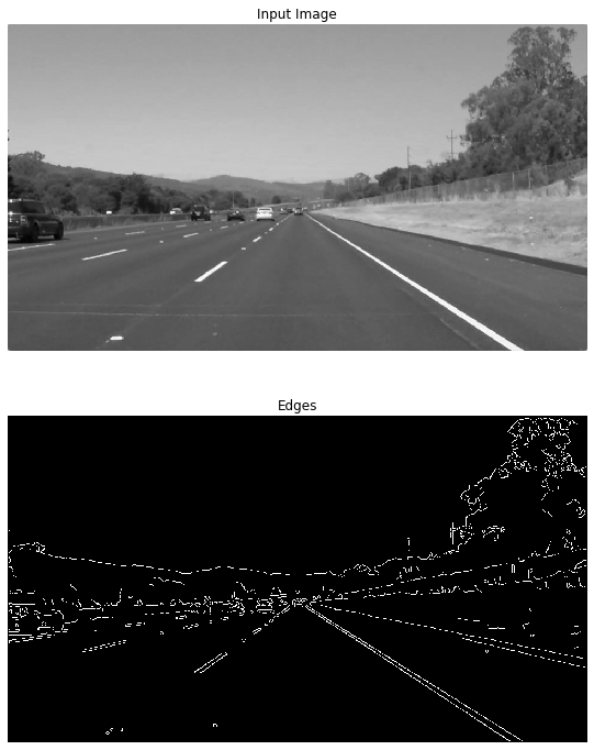
  • Edge detection
  • Extracting Region of Interest (ROI)
  • Fitting lines using Hough Transform

What did I learn?

• Implement Gaussian filter

• Implement Gradient and calculate it's magnitude and direction of each pixel.

• NMS steps:

  • Round the gradient direction to the nearest 45 degrees, corresponding to the use if an 8-conntected neighbourhood. $[0,45,90,135,180,225,270,315]$
  • Compare the edge strength of the current pixel with the edge strength of the pixel along with positive and negative geadient directions
  • If the edge strength of the current pixel if the largest, then preserve the value of the edge strength. If not, suppress (i.e. remove) the value.

• Hough Transform steps:

  • Find edges using Canny edge detector
  • Map edge points to Hough Space (r-theta coordinate)
  • Store mapped points in accumulator
  • Interpretate the accumulator to yield lines of infinite length
  • Converse infinite lines to finite lines
  • Reference

Pictures
Smooth
Grdient of x and y
NMS
Double Thresholding
Edge tracking by hysterisis
Edge detection
ROI
Hough transform

hw3 - Panorama - Image stitching [link]

(Lecture 04-06)

• Harris corner detector
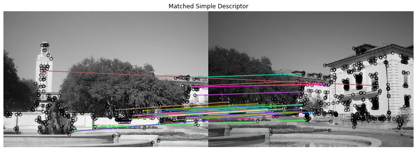
• Describing and Matching Keypoints
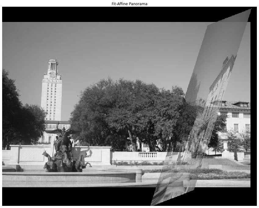
• Transformation Estimation
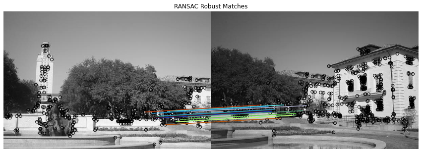
• RANSAC
• Histogram of Oriented Gradients (HOG)
• Better Image Merging - Linear Blending
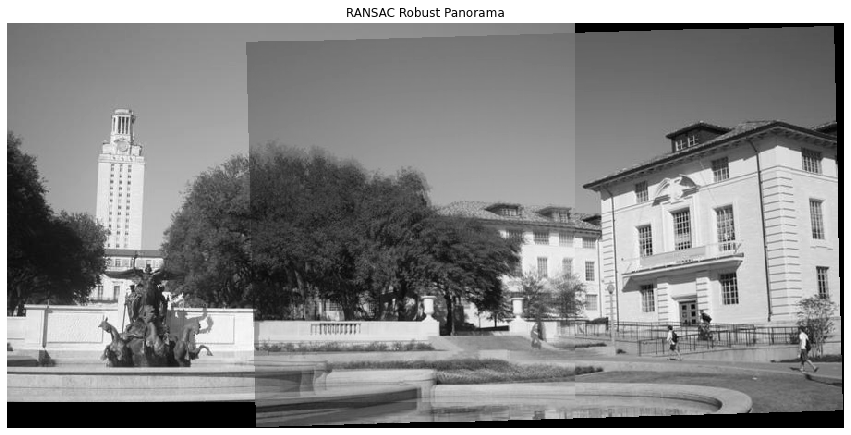
• Stitching Multiple Images

What did I learn?

• Harris corner detector

  • A method to get keypoints of the image.
  • Steps:
    1. Compute Ix and Iy derivatives of an image.
    2. Compute product of Ix^2/ Iy^2/ IxIy at each pixel
    3. Apply Gaussian smooth to 2. to get Sxx/ Syy/ Sxy
    4. Compute matrix M at each pixel and eigen value of M
    5. Compute response value R at each pixel, where R = Det(M)-k(Trace(M)^2)
    6. Use function corner_peaks from skimage.feature to get local maxima of response map by performing NMS and localize keypoints

• Describing and Matching Keypoints

  • Creating descriptors
    • Give each keypoints a patch
    • Normalize patch and then flattening into a 1D array
  • Matching descriptors
    • Calculate Euclidean distance between all pairs of descriptors form image1 to image2 (use scipy.spatial.distance.cdist(desc1, desc2, 'euclidean'))
    • Store 'match descriptors', if (first-closest pairs/ second-closest pairs) < threshold, then first-closest pairs is match

• Transformation Estimation

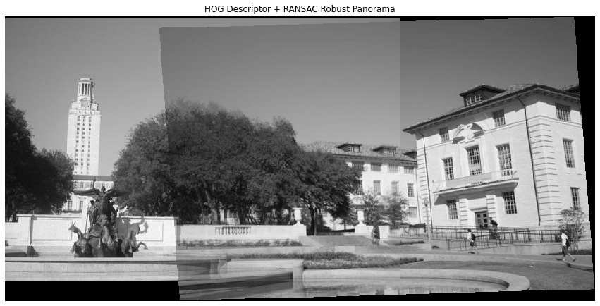
  • Use least square to calculate affine transformation matrix H letting p2*H = p1 (use np.linalg.lstsq)

• RANSAC

  • Steps:
    1. Given parameters:
       • n_iters: number of iterations
       • threshold: limitation for inliers
    2. Select a random set of matches
    3. Compute affine transformation matrix letting p2*H = p1 (use np.linalg.lstsq)
    4. Compute the number of inliers via Euclidean distance within the threshold (use np.linalg.norm(...ord=2))
    5. Keep the model with the most number of inliers
    6. Re-compute least-squares estimate on all of the inliers

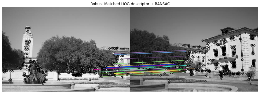
• Histogram of Oriented Gradients (HOG)

  • A method to describe keypoint
  • Steps:
    1. Compute the gradient image in x and y directions
       • Use the sobel filter provided by skimage.filters
    2. Compute gradient histograms
       • Divide image into cells, and calculate histogram of gradients in each cell
    3. Flatten block of histograms into feature vector
    4. Normalize flattened block by L2 norm

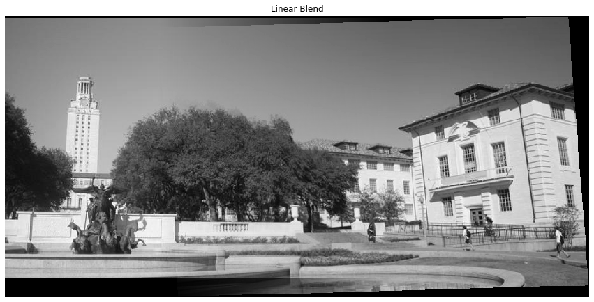
• Better Image Merging - Linear Blending

  • Define left and right margins for blending to occur between
  • Define a weight matrix for image 1 such that:
    • From the left of the output space to the left margin the weight is 1
    • From the left margin to the right margin, the weight linearly decrements from 1 to 0
  • Define a weight matrix for image 2 such that:
    • From the right of the output space to the right margin the weight is 1
    • From the left margin to the right margin, the weight linearly increments from 0 to 1
  • Apply the weight matrices to their corresponding images
  • Combine the images

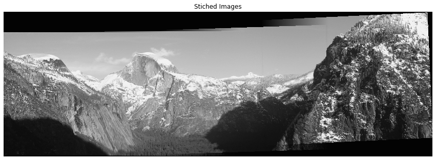
• Stitching Multiple Images

  • Combine the effects of multiple transformation matrices

Pictures
Harris corner response
Keypoinnts
Describing and matching keypoints (simple descriptor)
Transformation matrix H with least square method
Transformation matrix H with RANSAC method(Robust matches)
HOG descriptor
Better Image Merging - Linear Blending
Stitching Multiple Images

hw4 - Segmentation - clustering [link]

(Lecture09-10)

• Clustering Algorithm
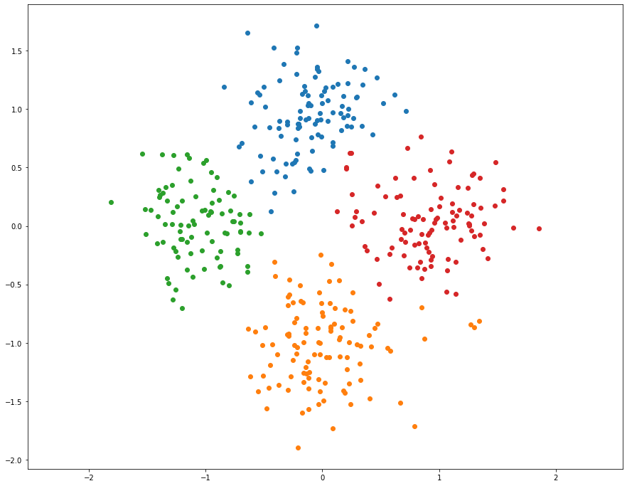
  • K-Means Clustering
  • K-Means Convergence
  • Heirarchical Agglomerative Clustering (HAC)
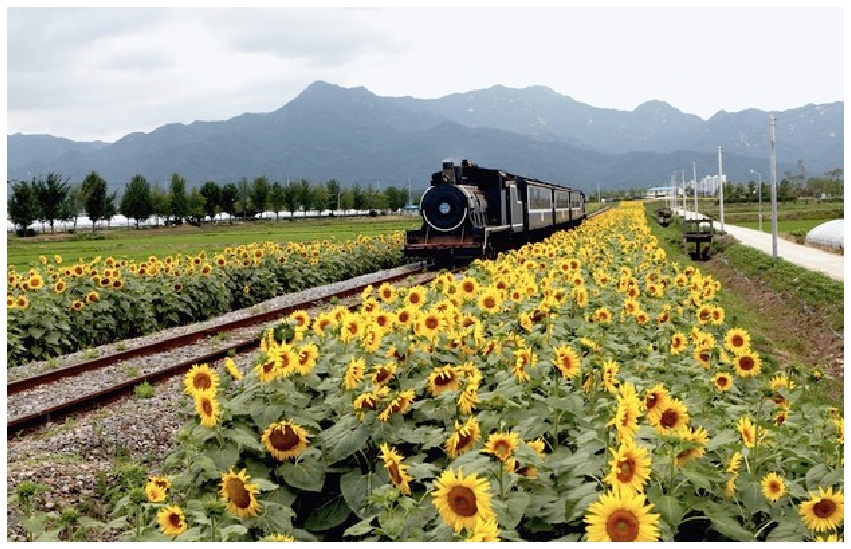
• Pixel-Level Features
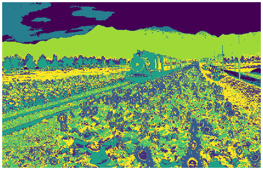
  • Color features
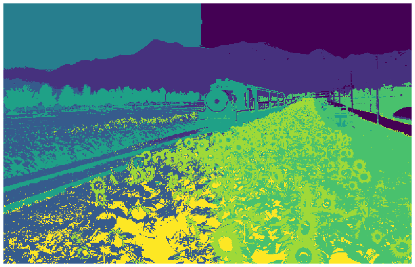
  • Color and Position Features
• Extra Credit: Implement Your Own Feature
• Quantitative Evaluation

What did I learn?

• K-Means Clustering

  • An algorithm for clustering by comparing distances between every point to clusters with the given parameter k.
  • k: number of clusters
  • Steps:
    1. Randomly initialize k cluster centers
    2. Assign each point to the closest center
    3. Recompute the new center of each cluster
    4. Stop if cluster assignments did not change
    5. Otherwise, go back to step 2

• Heirarchical Agglomerative Clustering (HAC)

  • An algorithm for clustering by merging the closest pair of clusters with the given parameter k.
  • k: number of clusters
  • Steps:
    1. Each point is its own cluster in the beginning
    2. Compute centers of every clusters
    3. Compute euclidean distances between every pairs of clusters (use pdist import from scipy.spatial.distance)
    4. Merge the closest pair of cluster as a new cluster
    5. Repeat steps 2-4 until k clusters remain

• How to improve the performance of the segmentation algorithm by modifying parameters.

Pictures
Clustering Algorithm

Pixel-Level Features
Original

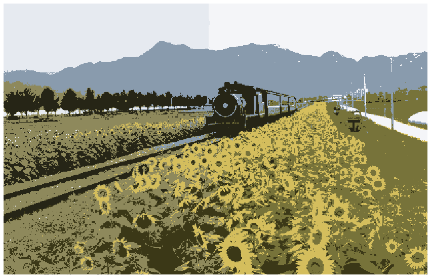
Color Features	Visualization

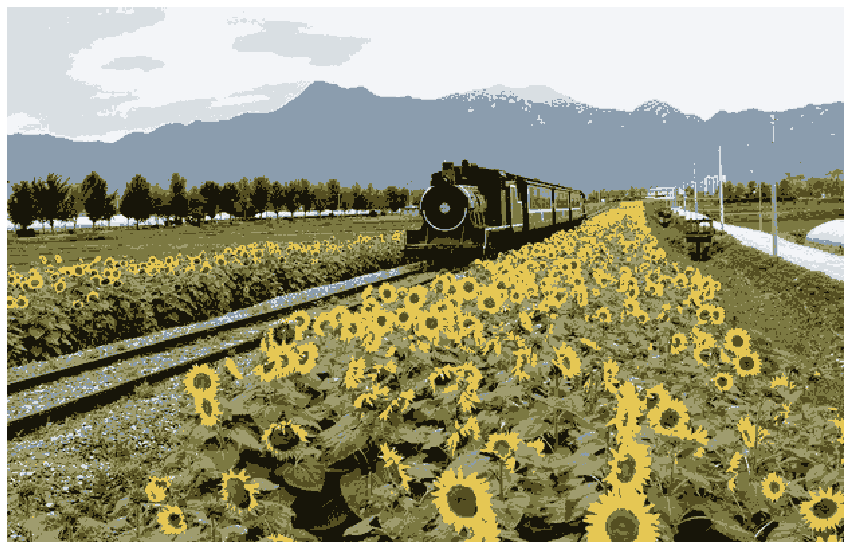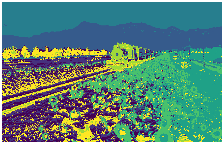
Color and Position Features	Visualization

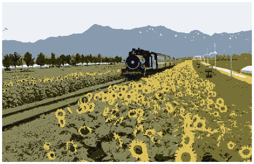
My Features	Visualization

Quantitative Evaluation

hw5 - Seam carving [link]

(Lecture11)

• Image Reducing using Seam Carving
  • Energy function
  • Compute cost
• Finding optimal seams
  • Backtrack seam
  • Reduce
• Image Enlarging
• Faster reduce
  • Reducing and enlarging on another image
  • Forward energy
• Object Removal

What did I learn?

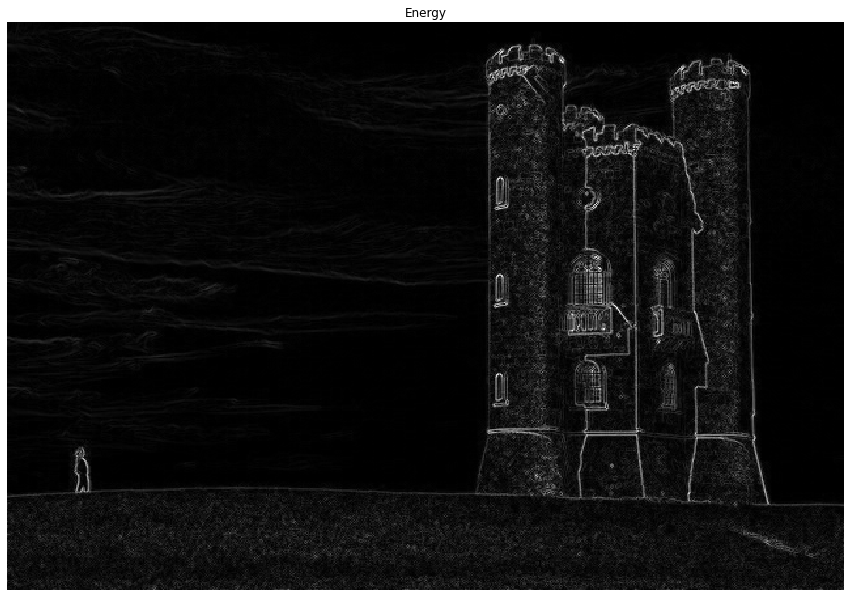
• Energy function

  • Energy map function can be represented as: (use np.gradient)
  • E(i,j) = E(i,j) = |Img(i,j)/dx|+|Img(i,j)/dy|

• Compute cost

  • Cost map function can be represented as:
  • M(i,j) = E(i,j) + min{M(i-1, j-1), M(i-1, j), M(i-1, j+1)}

• Backtrack seam

  • A strategy to find the seam from the last row to the top row

• Reduce

  • Steps:
    1. Compute the energy map
    2. Compute the cost map and paths direction at each pixel
    3. Compute the seam by backtracking
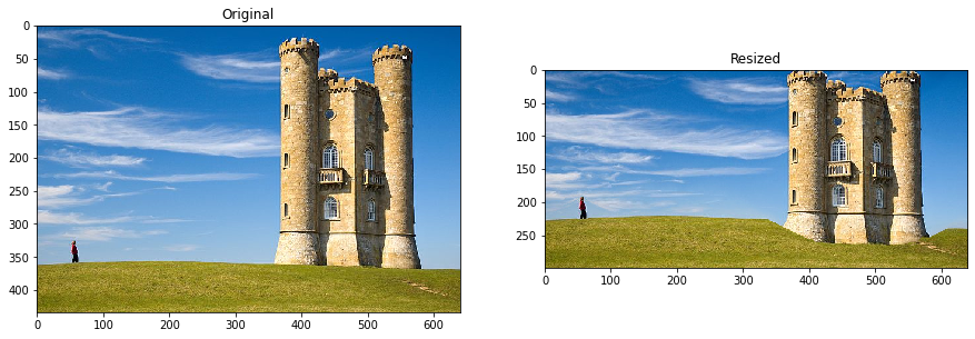
    4. Reduce the image by removing the seam
    5. Otherwise, go back to step 2
  • Fast reduce - only update the area of energy map that seam covered

• Enlarge

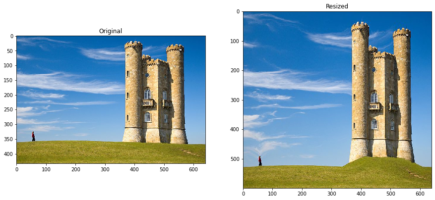
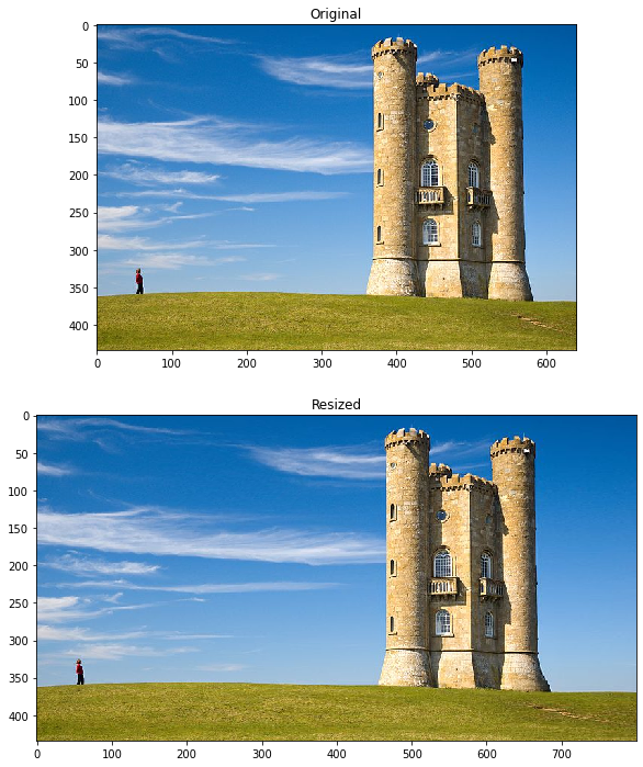
  • Enlarge the size of the image by duplicating the low-energy seams
  • We get the k seams to duplicate only one time to avoid repeatedly duplicating the same lowest-energy seam

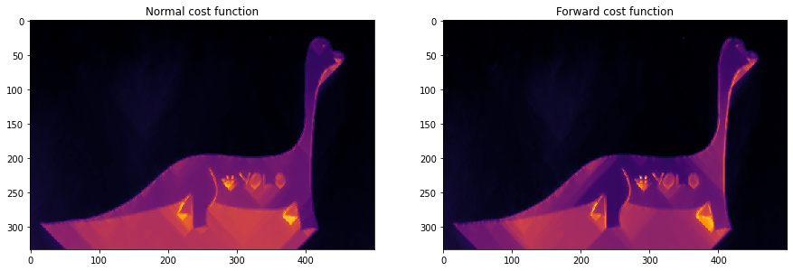
• Forward Cost

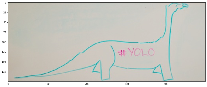
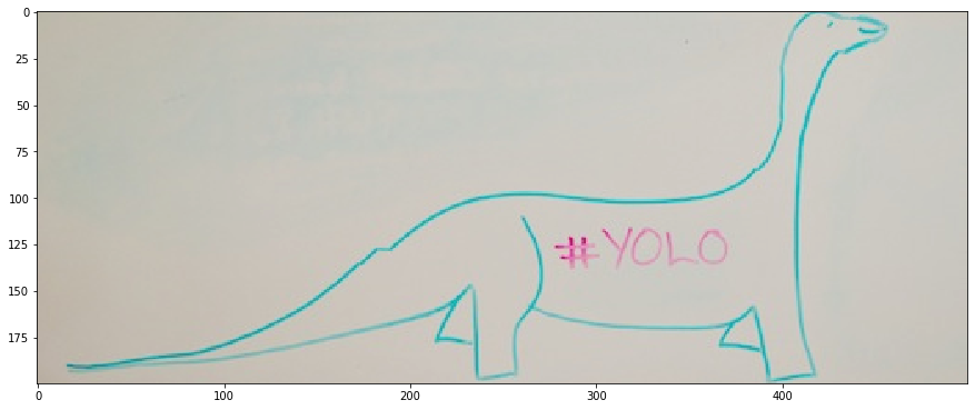
  • A strategy to avoid getting jagged edges
  • Focus on removing the seams that insert the least energy into the image rather than the least energy ones

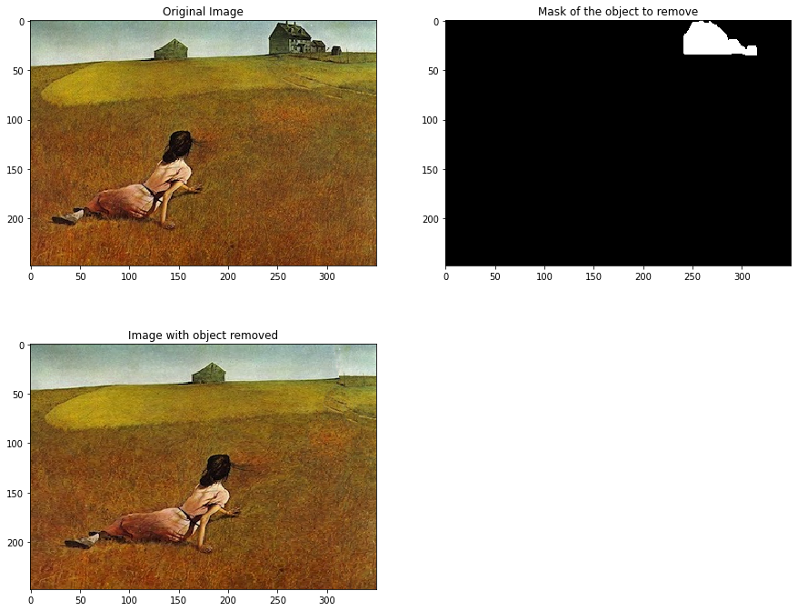
• Object removal

  • Steps:
    1. Reduce the image first by giving the mask
    2. Get weighted energy by giving the object area we want to remove less weight
    3. Enlarge image back to the original size

Pictures
Energy function

Compute cost (vertical)	Compute cost (horizontal)

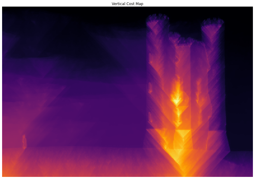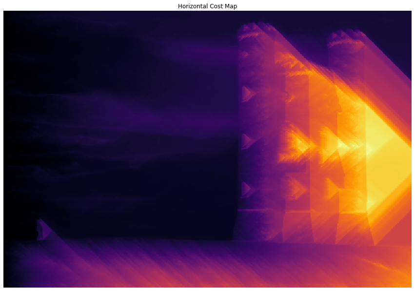Backtrack seam

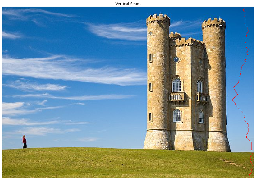Reduce (vertical)	Reduce (horizontal)
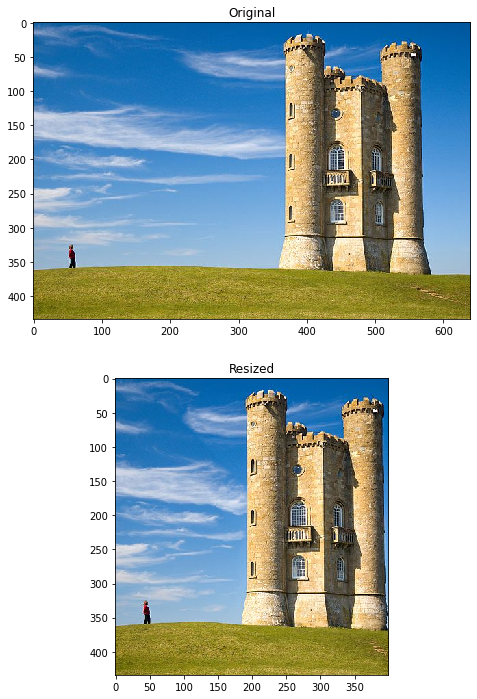Enlarge (vertical)	Enlarge (horizontal)

Forward cost map

Jagged edges	Smooth edges

Object Removal

hw6 - Object detection [link]

(Lecture12-14)

• Hog Representation
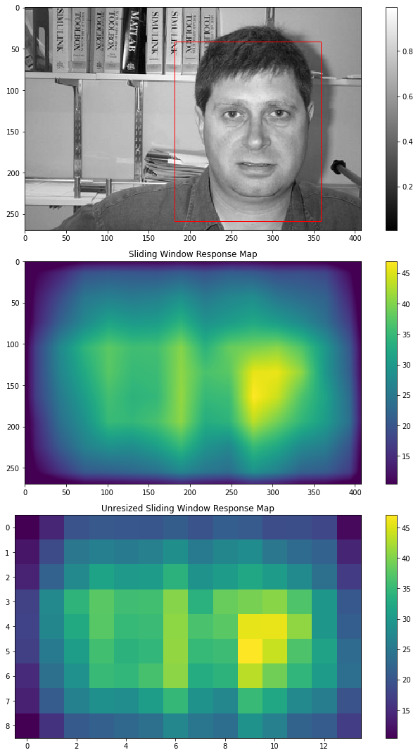
• Sliding Window
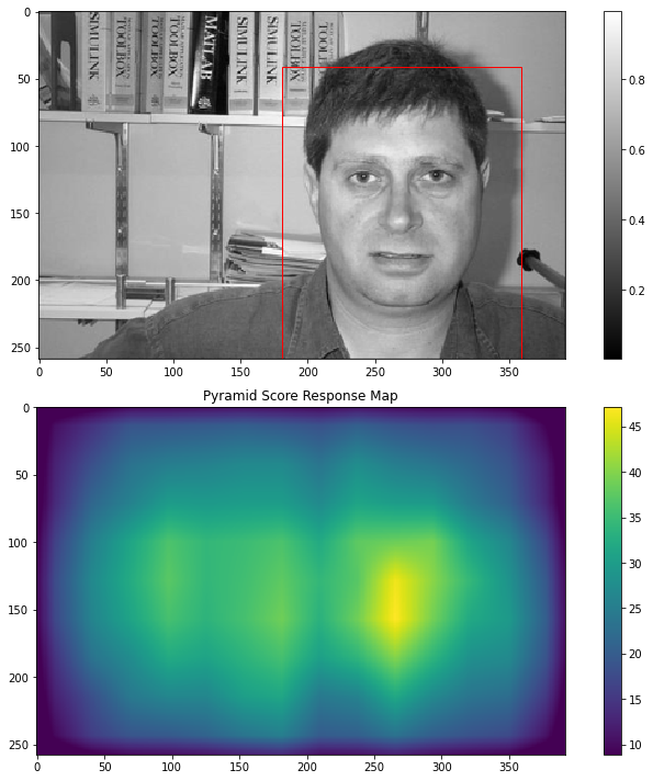
• Image Pyramids
• Deformable Parts Detection (DPM)
  • Compute displacement
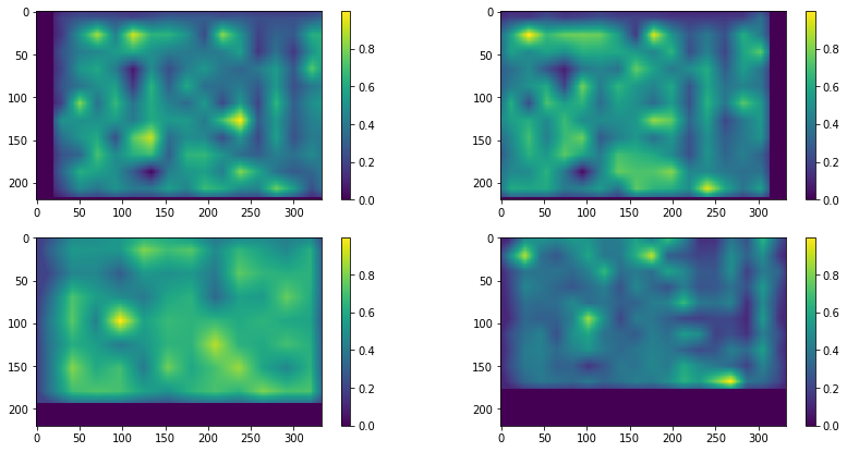
  • Shift heatmap
• Gaussian Filter
• K-Nearest Neighbors Classification
  • Cross validation on raw pixel features
  • Cross validation on HOG features

What did I learn?

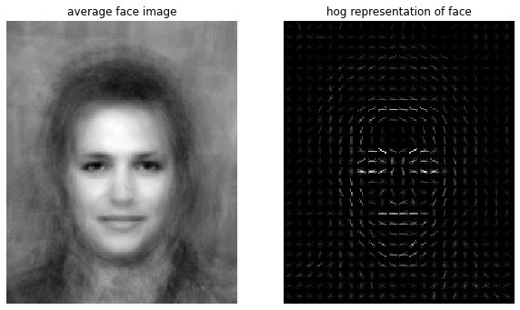
• Hog Representation

  • using skimage.feature.hog function

• Sliding Window

  • use in the template match
  • The hog score is computed as the dot product between the hog feature of the sliding window and the hog feature of the template
  • not working when the image's size is changed

• Image Pyramids

  • using template match in different scales
  • Solve the problems when image's size is changed

• Deformable Parts Detection (DPM)

  • Compute displacement
  • Shift heatmap (use interpolation.shift from scipy.ndimage)
  • Steps:
    1. Make sure there are labeled data of each parts, parts[i] = [[x1,y1], [x2,y2], [x3,y3]...]
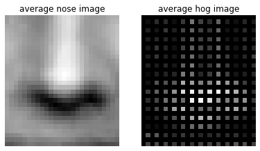
    2. Calculate averaging images and HOG features of each parts
    3. Calculate averaging displacements and standard deviations between each parts's center and face's center
    4. Calculate response map of face feature (sliding window + pyramids)
    5. Calculate response map of each parts (parts_feature)
    6. Move each parts[i] with displacement mu[i]

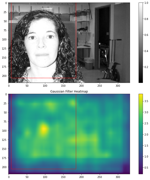
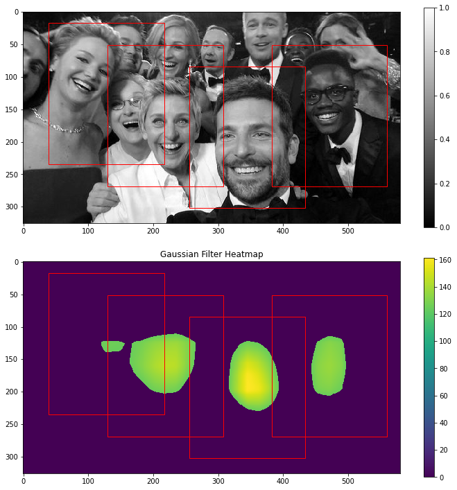
• Gaussian Filter

  • Apply gaussian filter to each parts' heatmap and add them to the heatmap of the face
  • The maximum value in combined heatmap is where the face located

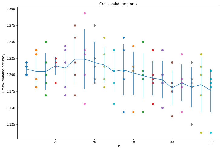
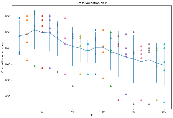
• K-Nearest Neighbors Classification/ Cross-validation

  • We have to find the best k for KNN algorithm by iterating k in each cross-validation fold
  • We perform cross-validation by spliting the dataset into N folds (N = 5 in this case)
  • Steps:
    1. Compute the distances between all features from X_train and from X_test
    2. Split the data into 5 folds to perform cross-validation
    3. Measure the mean accuracy for each value of k by averaging 5 accuracies
  • The accuracy performance of cross-validation on HOG features is much better than cross-validation on raw pixels

Pictures
Hog Representation
Sliding Window

Image Pyramids	Scaled image

Deformable Parts Detection (DPM)

Left eye	Right eye
Nose	Mouth
Shift-heatmap
Result	Detect multiple faces

K-Nearest Neighbors Classification/ Cross validation

Cross validation on raw pixels	Cross validation on HOG features