We have been approached by a Real Estate company in King-County, Settle WA who is looking to increase their profits and help their customers maximize the value of their homes by getting a better understanding of how different factors affect the price of a house. Our job is to analyze the data and create a presentation that explores the different types of features and how they affect house prices. We must then translate the findings into Recommendations and Actionable Insights that the company can use to decide which factors should be used to help maximize the profit and value of houses.
For this project I was provided with a Flatiron School variation of the 'kc_house_data', this dataset can also be found on Kaggle. In this repo you will also find copies of this data set at different stages of analysis:
- kc_house_data.csv: This is the original dataset provided.
- kc_cleaned: This is a copy of the dataset after the data cleaning stage of the analysis.
- kc_reg.csv: This is the final form of our data after cleaning and EDA. This is the dataset used to build Regression Models and draw final conclusions on my findings.
Like the datasets, there are 3 different notebooks containing my data analysis stages from data cleaning down to my conclusion:
- Data_Cleaning.ipynb: Like the file name this notebook contains all my data cleaning process, including, but not limited to, importing data, dealing with missing values, checking for duplicates, etc.
- EDA.ipynb: In this notebook I got the explore and understand the data better by, taking care Outliers, Feature Engineered new columns, dealing with Categorical columns, and answering questions to get more insight into the data.
- Regression_Notebook.ipynb: This final notebook cotains all my Regression Models and my final conclusions on the project.
An important aspect of data analysis is knowing how to ask the right questions to better understand the data. The following questions are designed to do that:
- Q1: What effect does Location have on house prices?
- Q2: Do renovated houses cost more?
- Q3: What is the impact of renovations on house grades and how do they both affect house prices?
- Q4: How does distance from a major city like Bellevue affect price?
As mentioned earlier the data cleaning process can be found in the Data_Cleaning.ipynb notebook. I started by importing the data with the use of Pandas and taking a look at columns and some of the rows the data entails. Along with this repo is a file that explains what the values in each Column represents. This is the list of what each Column represents:
- id - unique identified for a house
- dateDate - house was sold
- pricePrice - is prediction target
- bedroomsNumber - of Bedrooms/House
- bathroomsNumber - of bathrooms/bedrooms
- sqft_livingsquare - footage of the home
- sqft_lotsquare - footage of the lot
- floorsTotal - floors (levels) in house
- waterfront - House which has a view to a waterfront
- view - Has been viewed
- condition - How good the condition is ( Overall )
- grade - overall grade given to the housing unit, based on King County grading system
- sqft_above - square footage of house apart from basement
- sqft_basement - square footage of the basement
- yr_built - Built Year
- yr_renovated - Year when house was renovated
- zipcode - zip
- lat - Latitude coordinate
- long - Longitude coordinate
- sqft_living15 - The square footage of interior housing living space for the nearest 15 neighbors
- sqft_lot15 - The square footage of the land lots of the nearest 15 neighbors
With the use of one of Pandas many functions namely .shape I know that I am working with a dataset that contains 21597 Rows and 21 Columns. Once I got more acquainted to the dataset I moved on with the data cleaning process. which includes:
- Checking for duplicates in dataset.
- Checking for and replacing NULL Values.
- Transform Datatypes when necessary.
The next step in getting the data prepared for Modeling is to perform some Exploratory Data Analysis. This process consists of:
- Identifying Outliers in the dataset and dealing with them appropriately.
- Feature Engineering new columns when necessary.
- Checking if data is Normally Distributed
- Checking for Multicollinearity among predictors.
- Dealing with Categorical variables, and creating dummy variables when needed.
- Formulating questions to get Insights on the data.
- Feature Engineering: one of the first things I did in the EDA process is feature engineering 3 new columns, basement, renovated, and distance_from_bellevue.
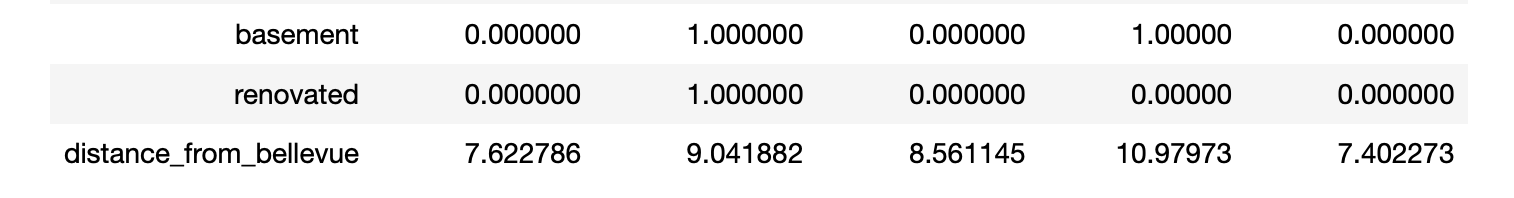

The 'basement' and 'renovated' where feature engineered from 'sqft_basement' and 'yr_renovated' respectively. Both columns where transformed to binary columns, 1 if a house has a basement or has been renovated and 0 if otherwise. The 'distance_from_bellevue' column was engineered a bit differently. I combined the 'lat' and 'long' columns to get the coordinates of each house, then I created a variable for Bellevue's coordinates as well. I then used the Haversine library to get the distance in miles of each house from Bellevue.
- Number of Bathrooms: After dealing with outliers in the dataset I decided to take a closer look at the bathrooms column.
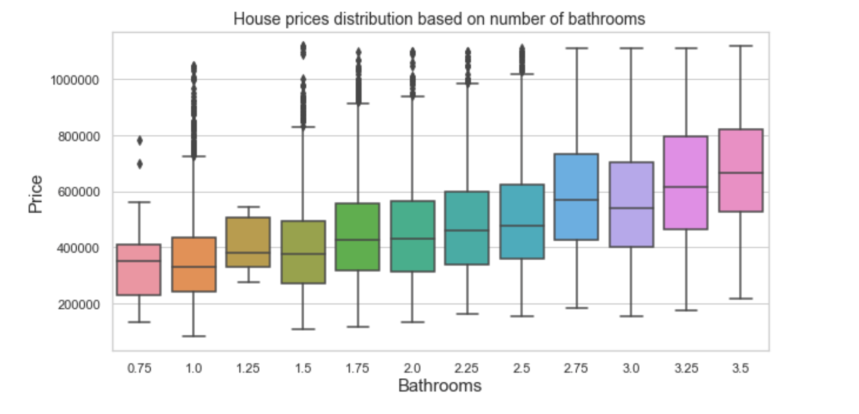

Upon closer look at each bathroom size you can see that there are bathrooms ending in 0.75/0.25, these aren't very realistic number when it comes to actual bathroom specs. By taking a closer look at the boxplot distribution of bathroom and price I was able to approximate these numbers with real bathroom specs that averaged around the same price, i.e, bathrooms ending in 0.75 where approximated to the next whole number.
-
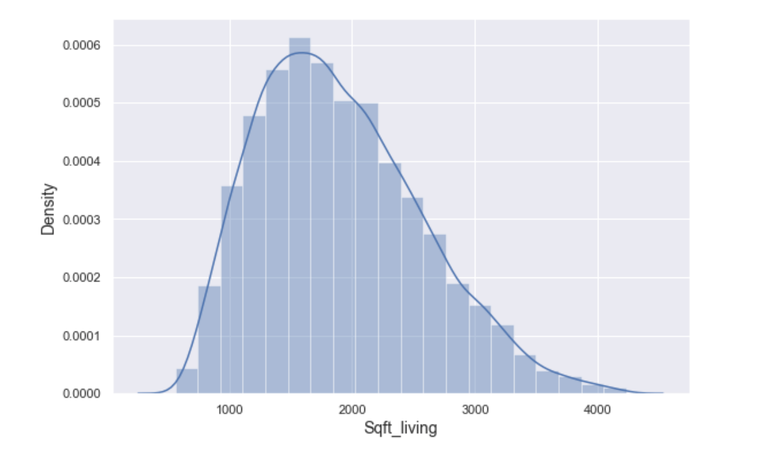
Distribution: Next I checked the distribution of each feature. Of all the features only 3 features(including price) where close to being normally distributed.
-
Multicollinearity: The next step in my EDA process was to check for multicollinearity among independent variables. Multicollinearity among independent features can have a negative impact on our regression models so it is best to get rid of highly correlated features.


For this dataset I chose 0.75 as the threshold for multicollinearity and if you take a close look at the heatmap you can see that 'sqft_living' and 'sqft_above' have a correlation of 0.82 which is higher than the set thershold. I decided to drop 'sqft_above' as it was a lot less correlated to our targer variable 'price'

- Dummy Variables: Before asking some questions to gain further insights on the data, I dealt with the Catergorical variables in the dataset

Asides from Waterfront, Basement, and Renovated(already 1's and 0's and don't need any further transformations) the image shows us all the categorical features present in the dataset. There are 2 types of Catergorical variables Norminal and Ordinal variables. Norminal variables are variables that have two or more categorical values, but do not have an intrinsic order. Ordinal variables like norminal variables have two or more categorical variables but unlike norminal, ordinal categories can be ordered or ranked. Of all the displayed categorical variables only 2 features were Norminal and need to be transformed through One-Hot Encoding.
The last act of my EDA process is to answer the questions defined earlier.
- Q1: What effect does Location have on house prices?
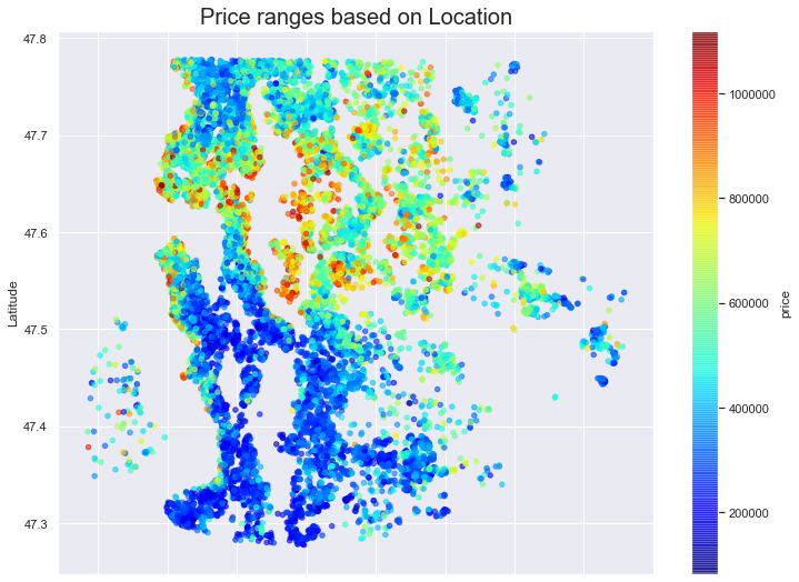

The further north we go the higher the price of a property. This could be for a number of reasons we will explore further later.
- Q2: Do renovated houses cost more?

It's very clear to see the difference in price of renovated house from houses that have not been renovated.
- Q3: What is the impact of renovations on house grades and how do they both affect house prices?
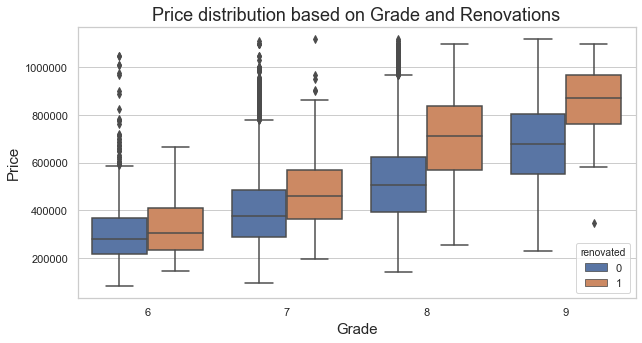

Just like the renovated graph we can see the houses that have been Renovated regardless of Grade cost.
- Q4: How does distance from a major city like Bellevue affect price?
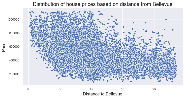

There is a negative relationship bwtween 'price' and 'distance_from_bellevue', which tells us the further away a property is from Bellevue the more the price decreases.
The final step is to build model with the improved data obtained from the data analysis process. In order to build a good Linear Regression model there are 3 assumptions to be met: Linearity, Normality, and Homoscedasticity. No single feature seem to make a very good Linear regression as most failed to mean 1 or more assumptions. The next course of action is to construct a Multiple Linear Regression Model.
Model Summary

The final model has a $ R^2 $ of 0.663, this tells us the the model explains 66% of the variability of the response data around it's mean.


Looking at the displot graph ans QQ plot we can see that the data is moderately normal.
- If a property is near a Waterfront we expect it to cost about 285,214 more.
- The price of a house decreases by 1,413 for every new construction made yearly.
- An increase in the Grade due to renovations can bring the house value up by 86,864.
- An increase in Lat is equivalent to an increase of 250,628 for a property.
- A sqft unit increase is equivalent to an increase of 122 in price
- The further away a house is from Bellevue city the less it cost, ie, 11,804 is lost the further away a property is from Bellevue.