![]()
Apygee (apogee + py) is a lightweight Python package for creating, manipulating and visualizing Kepler orbits.
pip install apygeeThe main export of Apygee is the Orbit class, which stores the keplerian elements and provides easy access to the astrodynamical properties of the orbit. It also contains methods for visualizing the orbit, and for performing mauevers in order to transfer to other orbits.
from apygee import Orbit, MU_EARTH

orbit = Orbit([2e6], mu=MU_EARTH)
print(orbit)
Orbit([a=2e+6, e=0, i=0, Ω=0, ω=0, θ=0], μ=3.99e+14, type='circular')
Apygee provides conversion functions between cartesian and keplerian elements, as provided by the exports kep_to_cart and cart_to_kep. The Orbit class also has a from_cart constructor to facilitate conversion.
For interactive versions, see the notebook in the examples directory.
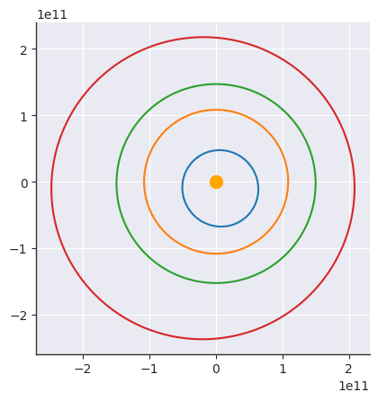
import matplotlib.pyplot as plt
from apygee import MERCURY, VENUS, EARTH, MARS

MERCURY.plot()
VENUS.plot()
EARTH.plot()
MARS.plot()

plt.scatter([0], [0], s=100, color="orange")
<matplotlib.collections.PathCollection at 0x7fc0896a9280>
import numpy as np
import matplotlib.pyplot as plt
from apygee import Orbit, MU_EARTH

orbit = Orbit([2e6, 0.45, np.pi / 3, 0, 0, np.pi / 2], mu=MU_EARTH)

# To plot in 3d, create a 3d axis before calling `.plot`
ax = plt.axes(projection="3d")
orbit.plot(show=["r", "r_p", "r_a"])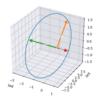
import matplotlib.pyplot as plt
from apygee import Orbit, MU_EARTH

orbit = Orbit([2e6, 0.45, np.pi / 3, np.pi / 2.5, np.pi * 0.8, np.pi / 2], mu=MU_EARTH)

# To plot in 3d, create a 3d axis before calling `.plot`
ax = plt.axes(projection="3d")
orbit.plot(show=["r_p", "r", "theta", "n", "omega", "x", "Omega"])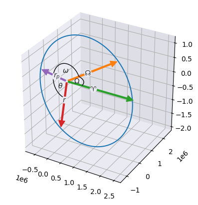
from apygee import Orbit, MU_EARTH

orbit = Orbit([2e6], mu=MU_EARTH)
orbit.visualize()
import numpy as np
import matplotlib.pyplot as plt
from apygee import Orbit, EARTH, MARS, MU_SUN
earth = Orbit([EARTH.a], mu=MU_SUN).at_theta(0)
mars = Orbit([MARS.a], mu=MU_SUN).at_theta(np.pi)
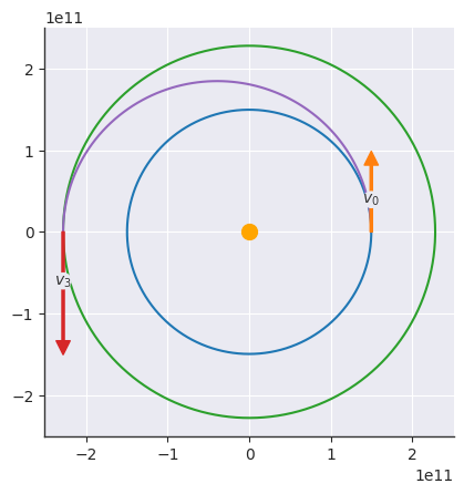
transfer = earth.hohmann_transfer(mars)
# Note: the velocities are *not* drawn to scale! Only the direction is "correct"
earth.plot(show=["v"], labels={"v": "$v_0$"})
mars.plot(show=["v"], labels={"v": "$v_3$"})
transfer.plot(thetas=np.linspace(0, np.pi, 100))
plt.scatter([0], [0], s=100, color="orange")
v0 = earth.at_theta(0).v_vec
v1 = transfer.at_theta(0).v_vec
dv1 = np.linalg.norm(v1 - v0)
print(f"Δv1 = {dv1/1e3:.2f} km/s")
v2 = transfer.at_theta(np.pi).v_vec
v3 = mars.at_theta(np.pi).v_vec
dv2 = np.linalg.norm(v3 - v2)
print(f"Δv2 = {dv2/1e3:.2f} km/s")
dv = dv1 + dv2
print(f"Total Δv = {dv/1e3:.2f} km/s")
dt = transfer.at_theta(np.pi).t - transfer.at_theta(0).t
print(f"Δt = {dt/3600/24:.2f} days")Δv1 = 2.94 km/s
Δv2 = 2.65 km/s
Total Δv = 5.59 km/s
Δt = 258.86 days
import numpy as np
import matplotlib.pyplot as plt
from apygee import Orbit, EARTH, MARS, MU_SUN
earth = Orbit([EARTH.a], mu=MU_SUN).at_theta(0)
mars = Orbit([MARS.a], mu=MU_SUN).at_theta(np.pi)
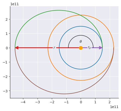
[transfer1, transfer2] = earth.bielliptic_transfer(mars, ra=mars.ra * 2)
earth.plot()
mars.plot()
transfer1.plot(thetas=np.linspace(0, np.pi, 100), theta=np.pi, show=["r", "r_p", "theta"])
transfer2.plot(thetas=np.linspace(np.pi, 2 * np.pi, 100))
plt.scatter([0], [0], s=100, color="orange", zorder=3)
v0 = earth.at_theta(0).v_vec
v1 = transfer1.at_theta(0).v_vec
dv1 = np.linalg.norm(v1 - v0)
print(f"Δv1 = {dv1/1e3:.2f} km/s")
v2 = transfer1.at_theta(np.pi).v_vec
v3 = transfer2.at_theta(np.pi).v_vec
dv2 = np.linalg.norm(v3 - v2)
print(f"Δv2 = {dv2/1e3:.2f} km/s")
v4 = transfer2.at_theta(0).v_vec
v5 = mars.at_theta(2 * np.pi).v_vec
dv3 = np.linalg.norm(v5 - v4)
print(f"Δv3 = {dv3/1e3:.2f} km/s")
dv = dv1 + dv2 + dv3
print(f"Total Δv = {dv/1e3:.2f} km/s")Δv1 = 6.77 km/s
Δv2 = 1.94 km/s
Δv3 = 3.73 km/s
Total Δv = 12.44 km/s
from itertools import product
from apygee import Orbit, EARTH, MU_SUN
import matplotlib.pyplot as plt
import numpy as np
plt.style.use(
[
"seaborn-v0_8-darkgrid",
{
"axes.spines.top": False,
"axes.spines.right": False,
"axes.edgecolor": (0.2, 0.2, 0.2),
"axes.linewidth": 1,
"xtick.major.size": 3.5,
"ytick.major.size": 3.5,
},
]
)
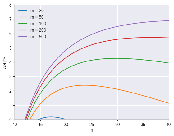
def hohmann(n, m):
r1 = EARTH.a
r2 = n * r1
orbit1 = Orbit([r1], MU_SUN)
orbit2 = Orbit([r2], MU_SUN)
transfer = orbit1.hohmann_transfer(orbit2)
v0 = orbit1.at_theta(0).v_vec
v1 = transfer.at_theta(0).v_vec
dv1 = np.linalg.norm(v1 - v0)
v2 = transfer.at_theta(np.pi).v_vec
v3 = orbit2.at_theta(np.pi).v_vec
dv2 = np.linalg.norm(v3 - v2)
return dv1 + dv2
def bielliptic(n, m):
r1 = EARTH.a
r2 = n * r1
ra = m * r1
orbit1 = Orbit([r1], MU_SUN)
orbit2 = Orbit([r2], MU_SUN)
[transfer1, transfer2] = orbit1.bielliptic_transfer(orbit2, ra=ra)
v0 = orbit1.at_theta(0).v_vec
v1 = transfer1.at_theta(0).v_vec
dv1 = np.linalg.norm(v1 - v0)
v2 = transfer1.at_theta(np.pi).v_vec
v3 = transfer2.at_theta(np.pi).v_vec
dv2 = np.linalg.norm(v3 - v2)
v4 = transfer2.at_theta(0).v_vec
v5 = orbit2.at_theta(2 * np.pi).v_vec
dv3 = np.linalg.norm(v5 - v4)
return dv1 + dv2 + dv3
ns = np.linspace(10, 40, 100)
ms = np.array([20, 50, 100, 200, 500])
def filter_nm(x):
[n, m] = x
if not m > n:
return False
if not (n > 1 and m > 1):
return False
return True
nns = []
mms = []
GGs = []
for n, m in filter(filter_nm, product(ns, ms)):
dvh = hohmann(n, m)
dvb = bielliptic(n, m)
G = -(dvb - dvh) / dvh * 100
nns.append(n)
mms.append(m)
GGs.append(G)
res = np.vstack([nns, mms, GGs]).T
for m in np.unique(res[:, 1]):
mask = res[:, 1] == m
plt.plot(res[mask, 0], res[mask, 2], label=f"m = {m:.0f}")
plt.xlabel("n")
plt.ylabel("ΔG [%]")
plt.xlim([10, 40])
plt.ylim([0, 8])
plt.legend()<matplotlib.legend.Legend at 0x7fc07ec34b30>
import numpy as np
import matplotlib.pyplot as plt
from apygee import Orbit, EARTH, MARS, MU_SUN
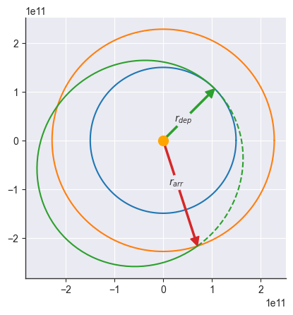
theta_dep = np.pi / 4
theta_arr = 8 * np.pi / 5
earth = Orbit([EARTH.a], mu=MU_SUN)
mars = Orbit([MARS.a], mu=MU_SUN)
transfer = earth.coplanar_transfer(mars, theta_dep, theta_arr)
earth.plot()
mars.plot()
transfer.plot(
thetas=np.linspace(theta_dep, theta_arr, num=100) - transfer.omega,
theta=theta_dep - transfer.omega,
labels={"r": r"$r_{dep}$"},
show=["r"],
c="tab:green",
)
transfer.plot(
thetas=np.linspace(theta_arr, theta_dep + 2 * np.pi) - transfer.omega,
theta=theta_arr - transfer.omega,
labels={"r": r"$r_{arr}$"},
show=["r"],
c="tab:green",
ls="--",
)
plt.scatter([0], [0], s=100, color="orange", zorder=3)<matplotlib.collections.PathCollection at 0x7fc07ec355b0>
import matplotlib.pyplot as plt
from apygee import Orbit, MU_EARTH

theta = np.pi / 4
dtheta = np.pi

orbit = Orbit([2e6], mu=MU_EARTH)
orbit.plot(theta=theta, show=["r"], label="orbit")

# Providing `dv` as a scalar requires passing the angle `x` (see below for visualization)
transfer = orbit.impulsive_shot(dv=3e3, x=np.pi / 3, theta=theta)
transfer.plot(thetas=np.linspace(transfer.theta, transfer.theta + dtheta, 100), label="transfer")

# Alternatively, provide `dv` as a vector:
theta2 = dtheta + (theta - transfer.omega)
transfer2 = transfer.impulsive_shot(dv=[3e3, 1e3, 2e3], theta=theta2)
transfer2.plot(theta=transfer2.theta, show=["r"], label="transfer2")

plt.scatter([0], [0], s=100, color="orange", zorder=3)
plt.xlim(np.array(plt.xlim()) * [1, 1.4])
plt.legend(loc="upper right")
<matplotlib.legend.Legend at 0x7fc07ecdd010>
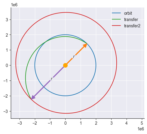
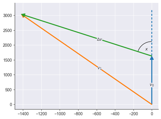
The angle x is measured between the dv vector and v0, which we can visualize using the utility functions plot_vector and plot_angle:
from apygee.plot import plot_vector, plot_angle
from apygee.utils import angle_between, rotate_vector

orbit = Orbit([150e6], MU_EARTH)
theta = 0
x = 0.789
dv = 2e3

v0 = orbit.at_theta(theta).v_vec

uv = v0 / np.linalg.norm(v0)
dv_vec = rotate_vector(uv, orbit.h_vec, x) * dv
v1 = v0 + dv_vec

plot_vector(v0, text="$v_0$")
plot_vector(v1, text="$v_1$")
plot_vector(dv_vec, origin=v0, text=r"$\Delta v$")

plot_angle(v0, dv_vec, origin=v0, text="$x$")
plot_vector(
    v0,
    origin=v0,
    arrow_kwargs=dict(arrowstyle="-", color="#1f77b4", lw=2, ls=(0, (2, 2.5))),
)

print(angle_between(dv_vec, v0), x)
0.789 0.789
Contributions are welcome! For bug reports or feature requests, please submit an issue on the GitHub repository.
This course is mainly based on the courses "Fundamentals of Astrodynamics" and "Numerical Astrodynamics" that I attended at TU Delft, taught by the wonderful Kevin Cowan. In addition, the following sources are used:
- Orbital Mechanics & Astrodynamics. (n.d.). Retrieved from https://orbital-mechanics.space/
- Bate, R. R., Mueller, D. D., White, J. E., & Saylor, W. W. (2020). Fundamentals of Astrodynamics (Revised and updated second edition). Dover Publications, Inc.
- Curtis, H. D. (2020). Orbital Mechanics for Engineering Students (4th ed.). Elsevier. ISBN 978-0-08-102133-0.
- de Pater, I., & Lissauer, J. J. (2015). Planetary Sciences (2nd ed.). Cambridge: Cambridge University Press.
This project is licensed under the terms of the MIT license.