An Adaptive Network with Consecutive and Intertwined Slices for Real-world Time-Series Forecasting

This is the origin Pytorch implementation of AdaNS in the following paper: [An Adaptive Network with Consecutive and Intertwined Slices for Real-world Time-Series Forecasting] (Manuscript submitted to INS).

The Entire Architecture of AdaNS

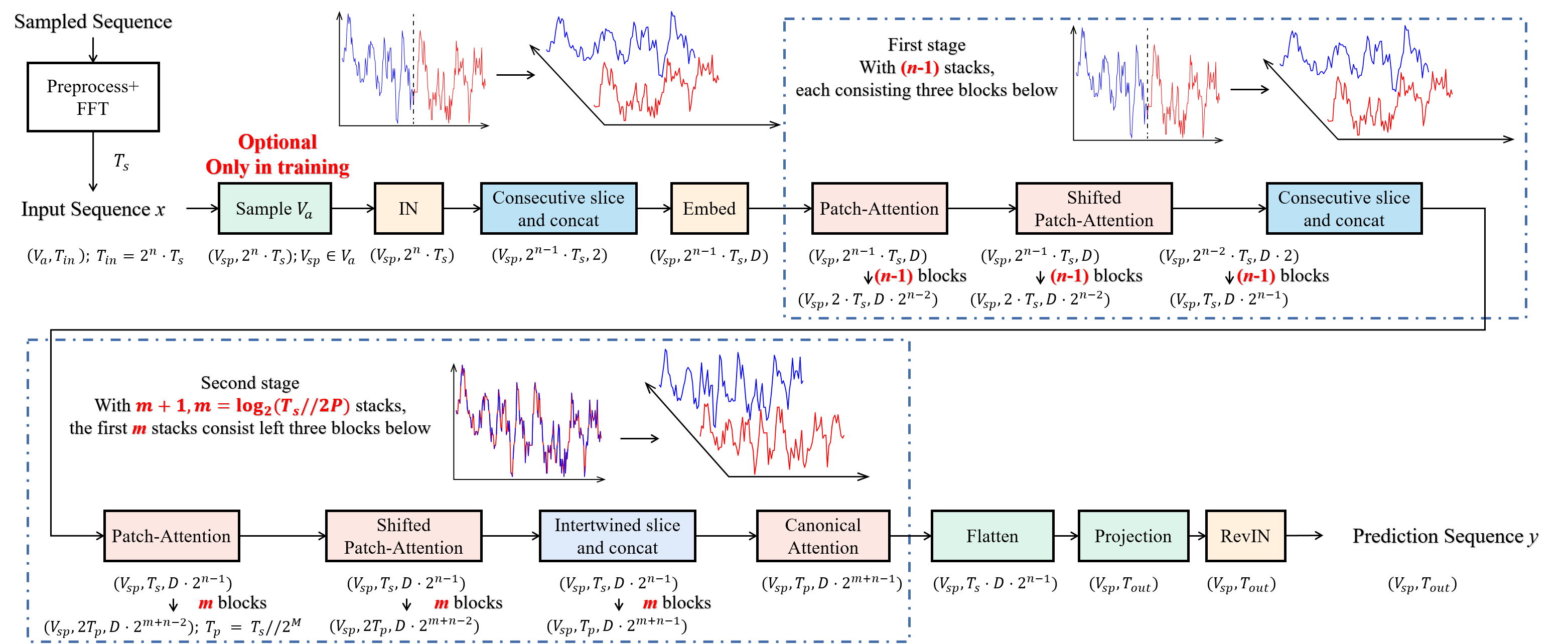
The backbone of AdaNS can be divided into two stages, as shown in Figure 1. The input sequence length is assumed to $2^n \cdot T_s$ and variables are categorized into different groups according to different $T_s$. We only discuss the network for an arbitrary variable group with variable numbers $V_a (V_a ≤ V)$ as the networks for other groups are similar. Moreover, we have also mentioned that the input sequence is sliced by half, concatenated to acquire features and embedded to prepare for feature extraction in AdaNS with FVS feature selection strategy. Then, the embedded input tensor is sent to the first stage for universally periodic feature extraction.

Figure 1. An overview of AdaNS. The size of the feature map is given under every block. The components in the upper dashed box belong to the first stage while those in the lower dashed box are the components of the second stage. The skip-connections with moving average, which are employed in the attention blocks, are omitted. The examples of consecutive slice and intertwined slice processes are given on the top of the corresponding blocks.

Requirements

Python 3.8.8
matplotlib == 3.3.4
numpy == 1.20.1
pandas == 1.2.4
scipy == 1.9.0
scikit_learn == 0.24.1
torch == 1.11.0

Dependencies can be installed using the following command:

pip install -r requirements.txt

Data

ETT, ECL, Traffic and weather dataset were acquired at: here. Solar dataset were acquired at: here. M4 dataset was acquired at: M4. Ship dataset was in ./data/Ship/ and its raw data was in https://coast.noaa.gov/hthata/CMSP/AISDataHandler/2022/index.html, the raw data of Air dataset was acquired at: https://archive.ics.uci.edu/dataset/360/air+quality and the raw data of Light dataset was acquired at: https://archive.ics.uci.edu/dataset/374/appliances+energy+prediction.

Data Preparation

After you acquire raw data of all datasets, please separately place them in corresponding folders at ./data.

We place ETT in the folder ./ETT-data, ECL in the folder ./electricity and weather in the folder ./weather of here (the folder tree in the link is shown as below) into folder ./data and rename them from ./ETT-data,./electricity, ./traffic and ./weather to ./ETT, ./ECL, ./Traffic and./weather respectively. We rename the file of ECL/Traffic from electricity.csv/traffic.csv to ECL.csv/Traffic.csv and rename its last variable from OT/OT to original MT_321/Sensor_861 separately.

The folder tree in https://drive.google.com/drive/folders/1ZOYpTUa82_jCcxIdTmyr0LXQfvaM9vIy?usp=sharing:
|-autoformer
| |-ETT-data
| | |-ETTh1.csv
| | |-ETTh2.csv
| | |-ETTm1.csv
| | |-ETTm2.csv
| |
| |-electricity
| | |-electricity.csv
| |
| |-traffic
| | |-traffic.csv
| |
| |-weather
| | |-weather.csv

We place Solar in the folder ./financial of here (the folder tree in the link is shown as below) into the folder ./data and rename them as ./Solar respectively.

The folder tree in https://drive.google.com/drive/folders/1Gv1MXjLo5bLGep4bsqDyaNMI2oQC9GH2?usp=sharing:
|-dataset
| |-financial
| | |-solar_AL.txt

We place Air/Light in Air/Light (the folder trees in the links are shown as below) into the folder ./data/Air/./data/Light.

The folder tree in https://archive.ics.uci.edu/dataset/360/air+quality:
|-air+quality
| |-AirQualityUCI.csv
| |-AirQualityUCI.xlsx

The folder tree in https://archive.ics.uci.edu/dataset/374/appliances+energy+prediction:
|-appliances+energy+prediction
| |-energydata_complete.csv

As for M4 dataset, we place the folders ./Dataset and ./Point Forecasts of M4 (the folder tree in the link is shown as below) into the folder ./data/M4. Moreover, we unzip the file ./Point Forecasts/submission-Naive2.rar to the current directory.

The folder tree in https://drive.google.com/drive/folders/1Gv1MXjLo5bLGep4bsqDyaNMI2oQC9GH2?usp=sharing:
|-M4-methods
| |-Dataset
| | |-Test
| | | |-Daily-test.csv
| | | |-Hourly-test.csv
| | | |-Monthly-test.csv
| | | |-Quarterly-test.csv
| | | |-Weekly-test.csv
| | | |-Yearly-test.csv
| | |-Train
| | | |-Daily-train.csv
| | | |-Hourly-train.csv
| | | |-Monthly-train.csv
| | | |-Quarterly-train.csv
| | | |-Weekly-train.csv
| | | |-Yearly-train.csv
| | |-M4-info.csv
| |-Point Forecasts
| | |-submission-Naive2.rar

Then you can run ./data/preprocess.py to preprocess the raw data of Air and Light datasets. We replace the missing values, which are tagged with -200 value, by the average values of normal ones. We remove the variable NMHC(GT) in Air dataset in that all data of thisvariable in test subset is missing. We remove two random variables, i.e., rv1 and rv2, in Light dataset. After you successfully run ./data/preprocess.py, you will obtain folder tree:

|-data
| |-Air
| | |-Air.csv
| | |-AirQualityUCI.csv
| | |-AirQualityUCI.xlsx
| |
| |-ECL
| | |-ECL.csv
| |
| |-ETT
| | |-ETTh1.csv
| | |-ETTh2.csv
| | |-ETTm1.csv
| | |-ETTm2.csv
| |
| |-Light
| | |-energydata_complete.csv
| | |-Light.csv
| |
| |-M4
| | |-Dataset
| | | |-Test
| | | | |-Daily-test.csv
| | | | |-Hourly-test.csv
| | | | |-Monthly-test.csv
| | | | |-Quarterly-test.csv
| | | | |-Weekly-test.csv
| | | | |-Yearly-test.csv
| | | |-Train
| | | | |-Daily-train.csv
| | | | |-Hourly-train.csv
| | | | |-Monthly-train.csv
| | | | |-Quarterly-train.csv
| | | | |-Weekly-train.csv
| | | | |-Yearly-train.csv
| | | |-M4-info.csv
| | |-Point Forecasts
| | | |-submission-Naive2.csv
| |
| |-Ship
| | |-Ship1.csv
| | |-Ship2.csv
| |
| |-Solar
| | |-solar_AL.txt
| |
| |-Traffic
| | |-Traffic.csv
| |
| |-weather
| | |-weather.csv

Baseline

We select seven typical deep time series forecasting models, i.e., MICN, Scaleformer, FiLM, PatchTST, Crossformer, DLinear and N-HiTS as baselines in multivariate/univariate forecasting experiments. Their source codes origins are given below:

Baseline	Source Code
MICN	https://github.com/wanghq21/MICN
Scaleformer	https://github.com/BorealisAI/scaleformer
FiLM	https://github.com/tianzhou2011/FiLM
PatchTST	https://github.com/yuqinie98/PatchTST
Crossformer	https://github.com/Thinklab-SJTU/Crossformer
DLinear	https://github.com/cure-lab/LTSF-Linear
N-HiTS	https://github.com/cchallu/n-hits

Moreover, the default experiment settings/parameters of aforementioned seven baselines are given below respectively:

Baselines	Settings/Parameters name	Descriptions	Default mechanisms/values
MICN	mode	The mode of trend prediction block	regre
	d_model	The number of hidden dimensions	512
	n_heads	The number of heads in multi-head attention mechanism	8
	d_layers	The number of decoder layers	1
	decomp_kernel	Decomposition kernel size	[17, 49]
	conv_kernel	Downsampling and upsampling convolution kernel size	[12, 16]
	isometric_kernel	Isometric convolution kernel size	[17, 49]
Scaleformer	scales	Scales in multi-scale	[16, 8, 4, 2, 1]
Scaleformer	scale_factor	Scale factor for upsample	2
FiLM	d_model	The number of hidden dimensions	512
	d_ff	Dimension of fcn	2048
	n_heads	The number of heads in multi-head attention mechanism	8
	e_layers	The number of encoder layers	2
	d_layers	The number of decoder layers	1
	modes1	The number of Fourier modes to multiply	32
PatchTST	patch_len	Patch length	16
PatchTST	stride	The stride length	8
Crossformer	seq_len	Segment length (L_seq)	6
	d_model	The number of hidden dimensions	64
	d_ff	Dimension of fcn	128
	n_heads	The number of heads in multi-head attention mechanism	2
	e_layers	The number of encoder layers	2
DLinear	moving_avg	The window size of moving average	25
N-HiTS	n_pool_kernel_size	Pooling kernel size	[4, 4, 4]
	n_blocks	The number of blocks in stacks	[1, 1, 1]
	n_x_hidden	Coefficients hidden dimensions	512
	n_freq_downsample	The number of stacks' coefficients	[60, 8, 1]

Usage

Commands for training and testing AdaNS of different datasets are respectively in the files ./scripts/<data>.sh.

More parameter information please refer to main.py.

We provide a complete command for training and testing AdaNS:

For multivariate forecasting:

python -u main.py --data <data> --features <features> --root_path <root_path> --Period_Times <Period_Times> --short_input_len <short_input_len> --pred_len <pred_len> --attn_pieces <attn_pieces> --learning_rate <learning_rate> --dropout <dropout> --Sample_strategy <Sample_strategy> --n_heads <n_heads> --sample_train <sample_train> --batch_size <batch_size> --train_epochs <train_epochs> --patience <patience> --itr <itr>

For univariate forecasting:

python -u main_M4.py --data <data> --features <features> --root_path <root_path> --Period_Times <Period_Times> --short_input_len <short_input_len> --pred_len <pred_len> --attn_pieces <attn_pieces> --learning_rate <learning_rate> --dropout <dropout> --Sample_strategy <Sample_strategy> --n_heads <n_heads> --sample_train <sample_train> --batch_size <batch_size> --train_epochs <train_epochs> --patience <patience> --itr <itr>

Here we provide a more detailed and complete command description for training and testing the model:

Parameter name	Description of parameter
data	The dataset name
root_path	The root path of the data file
data_path	The data file name
features	The forecasting task. This can be set to `M`,`S` (M : multivariate forecasting, S : univariate forecasting
target	Target feature in `S` task
checkpoints	Location of model checkpoints
tuned_checkpoints	Location of tuned model checkpoints
sample_train	The length of sampled sequence to seek $f_s$ and $T_s$
lmb	𝜆, one of the hyper-parameters used in outlier filter(year=6.25, season=1600, month=129600)
c	One of the hyper-parameters used in outlier filter
piece_len	The length of Ts, acqured by latter codes
Period_Times	The value of I
Sample_strategy	Sampling strategy in SCMA
short_input_len	Short input length for variable
pred_len	Prediction sequence length
c_in	Input size
c_out	Output size
w_random	Whether to train with partial variables
rand_thres	Threshold variable number determining whether to use w_random
factor	b, used in the method of sampling variables during training for datasets with large variable numbers
d_model	The hidden dimension of model
attn_pieces	The number of patches
n_heads	The number of heads
attn_nums1	Attention blocks of the first stage, acquired adaptivity
attn_nums2	Attention blocks of the second stage, acquired adaptivity
dropout	Dropout
itr	Experiments times
train_epochs	Train epochs
batch_size	The batch size of training input data
patience	Early stopping patience
learning_rate	Optimizer learning rate
loss	Loss function
load_tuned	Whether to load the tuned checkpoints

Results

The experiment parameters of each dataset are formated in the files within the directory ./scripts/. You can refer to these parameters for experiments, and you can also adjust the parameters to obtain better mse and mae results or draw better prediction figures. We provide the commands for obtain the results of AdaNS with hyper-parameters fine-tuning of ETT datasets in the files ./scripts/Tuned.sh and the corresponding checkpoints in the directory ./tuned_checkpoints/.

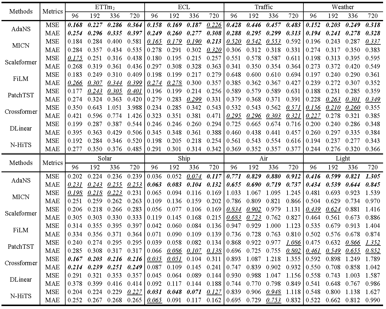
Figure 2. Multivariate forecasting results

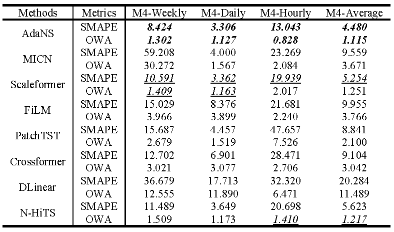
Figure 3. Univariate forecasting results

Contact

If you have any questions, feel free to contact Li Shen through Email (shenli@buaa.edu.cn) or Github issues. Pull requests are highly welcomed!

OrigamiSL / AdaNS