AFMF: Time Series Anomaly Detection Framework With Modified Forecasting

This is the origin Pytorch implementation of AFMF in the following paper: [AFMF: Time Series Anomaly Detection Framework With Modified Forecasting], which has been submitted to Knowledge-Based Systems.

Components of AFMF

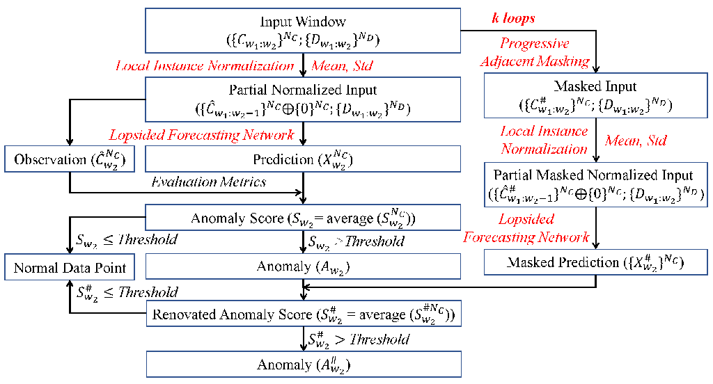
Figure 1. An overall algorithm flows of forecasting-based anomaly detection with AFMF. All of components changed/added by AFMF are emphasized in red. Oplus ($ \oplus $) refers to concatenation operation.

Local Instance Normalization (LIN)

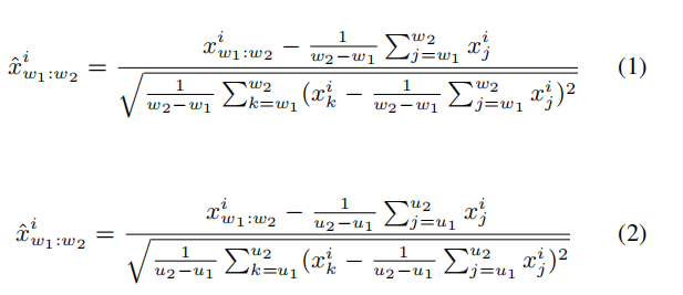
We propose Local Instance Normalization (LIN) which performs normalization per window $ x_{w_1:w_2}^N $ (Equation 1) as the preprocessing procedure to replace the conventional one which normalizes all data points with statistics of the entire dataset (Equation 2). $ [w_1,w_2] $ denotes time span of a certain window and $ [u_1,u_2] $ denotes time span of train subset. ${x}{w_1:w_2}^i$ refer to obversations in the dataset of the $ i $-th variate spanning this window and $ \hat{x}{w_1:w_2}^i $ are after normalization.

Lopsided Forecasting (LF)

As shown in Figure 2, inputs and outputs of Lopsided Forecasting (LF) are different from canonical forecasting format: (1) Inputs. Continuous variates are masked at prediction timestamp; Discrete variates are entirely inputted, including values at prediction timestamp. (2) Outputs. Only continuous variates are predicted. As the whole window, including observations of input and prediction parts, are all known in anomaly detection tasks, it is reasonable to utilize the value of discrete variates at prediction timestamps as inputs. When combining LF with LIN, we do not apply LIN to discrete variates, otherwise their implicit information will be damaged.

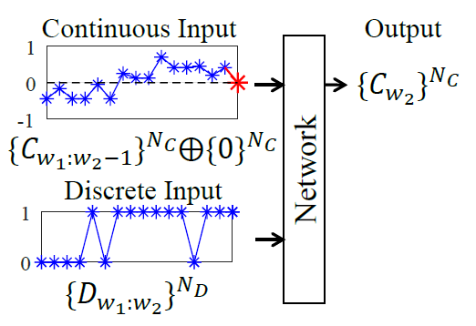
Figure 2. Lopsided forecasting only forecasts continuous variates $ \{C_{{w_2}}\}^{N_C} $ and its inputs extra include discrete variates at prediction timestamp $ \{D_{{w_2}}\}^{N_D} $. Additional zero $ \{0\}^{N_C} $ (red asterisk) concatenated with continuous inputs $ \{C_{{w_1:w_2-1}}\}^{N_C} $ is to ensure the same length with discrete inputs $ \{D_{{w_1:w_2}}\}^{N_D} $.

Progressive Adjacent Masking (PAM)

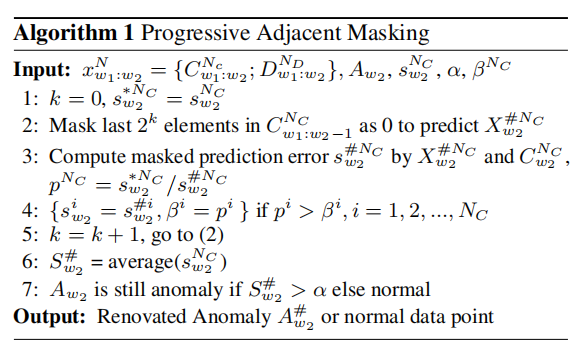
In practice, our proposed Progressive Adjacent Masking (PAM) is a progressive algorithm which avoids to decide the number of adjacent elements to mask. The pseudo-code of it is shown in Algorithm 1. $ N $ refers to the number of variates. $ A_{w_2} $ is certain anomaly detected by prediction error at $ w_2 $ ($ S_{w_2}^N $) and anomaly threshold ($ \alpha $) given by certain forecasting network. $ \beta^N $ is the hyper-parameter to initialize the decline ratio to determine whether the prediction error degradation is distinct enough to validate that the new prediction error after masking is more reliable.

Requirements

python == 3.8.8
numpy == 1.20.1
pandas == 1.2.4
scipy == 1.9.0
scikit_learn == 0.24.1
torch == 1.11.0
torch-cluster == 1.6.0
torch-geometric == 2.1.0.post1
torch-scatter == 2.0.9
torch-sparse == 0.6.15
torch-spline-conv == 1.2.1

Dependencies can be installed using the following command:

pip install -r requirements.txt

Data

SMD, MSL, SMAP, SMD datasets were acquired at datasets and SWaT, WADI can be requested at Itrust. MBA, UCR, NAB was acquired at TranAD datasets and MSDS can be requested at zenodo. Pruned and remedied {SMD, MSL, SMAP} were acquired at TranAD datasets.

Data Preparation

There are several versions of SWaT/WADI. We choose SWaT in the version of SWaT.A1 & A2_Dec 2015. The train subset is SWaT_Dataset_Normal_v1.xlsx and the test subset is SWaT_Dataset_Attack_v0. We choose WADI in the version of WADI.A2_19 Nov 2019. The train subset is WADI_14days_new.csv and the test subset is WADI_attackdataLABLE.csv. After you acquire raw data of all datasets, please separately place them in corresponding folders at ./AFMF/data. Then you can get the folder tree shown as below:

|-data
| | preprocess.py
| | data_loader.py
| |-MBA
| | |-labels.xlsx
| | |-test.xlsx
| | |-train.xlsx
| |
| |-MSDS
| | |-concurrent_data
| | | |-logs
| | | |-logs_aggregated_concurrent.csv
| | | |-metrics
| | | | |-wally113_metrics_concurrent.csv
| |
| |-MSL
| | |-test
| | | |-C-1.npy
| | |-train
| | | |-C-1.npy
| | |-labeled_anomalies.csv
| | |-MSL_test.npy
| | |-MSL_test_label.npy
| | |-MSL_train.npy
| |
| |-NAB
| | |-ec2_request_latency_system_failure.csv
| | |-labels.json
| |
| |-PSM
| | |-test.csv
| | |-test_label.csv
| | |-train.csv
| |
| |-SMAP
| | |-test
| | | |-P-1.npy
| | |-train
| | | |-P-1.npy
| | |-labeled_anomalies.csv
| | |-SMAP_test.npy
| | |-SMAP_test_label.npy
| | |-SMAP_train.npy
| |
| |-SMD
| | |-labels
| | | |-machine-1-1.txt
| | |-test
| | | |-machine-1-1.txt
| | |-train
| | | |-machine-1-1.txt
| | |-SMD_test.npy
| | |-SMD_test_label.npy
| | |-SMD_train.npy
| |
| |-SWaT
| | |-SWaT_Dataset_Attack_v0.xlsx
| | |-SWaT_Dataset_Normal_v1.xlsx
| |
| |-UCR
| | |-137_UCR_Anomaly_InternalBleeding18_2300_4485_4587.txt
| |
| |-WADI
| | |-WADI_14days_new.csv
| | |-WADI_attackdataLABLE.csv

Then you can run ./AFMF/data/preprocess.py to preprocess these raw data. Only raw data of SWaT, WADI and MSDS are preprocessed. We do not change any of their values but only remove useless information, e.g., blanks. We remove variates {'load.cpucore', 'load.min1', 'load.min5', 'load.min15'} in MSDS following TranAD. Names of variates are renamed for the convenience of variates classification in Lopsided Forecasting (LF). After you successfully run ./AFMF/data/preprocess.py, you will obtain folder tree:

|-data
| | preprocess.py
| | data_loader.py
| |-MBA
| | |-labels.xlsx
| | |-test.xlsx
| | |-train.xlsx
| |
| |-MSDS
| | |-concurrent_data
| | | |-logs
| | | |-logs_aggregated_concurrent.csv
| | | |-metrics
| | | | |-wally113_metrics_concurrent.csv
| | |-labels.csv
| | |-test.csv
| | |-train.csv
| |
| |-MSL
| | |-labels
| | | |-C-1.npy
| | |-test
| | | |-C-1.npy
| | |-train
| | | |-C-1.npy
| | |-labeled_anomalies.csv
| | |-MSL_test.npy
| | |-MSL_test_label.npy
| | |-MSL_train.npy
| |
| |-NAB
| | |-ec2_request_latency_system_failure.csv
| | |-labels.json
| |
| |-PSM
| | |-test.csv
| | |-test_label.csv
| | |-train.csv
| |
| |-SMAP
| | |-labels
| | | |-P-1.npy
| | |-test
| | | |-P-1.npy
| | |-train
| | | |-P-1.npy
| | |-labeled_anomalies.csv
| | |-SMAP_test.npy
| | |-SMAP_test_label.npy
| | |-SMAP_train.npy
| |
| |-SMD
| | |-labels
| | | |-machine-1-1.txt
| | |-test
| | | |-machine-1-1.txt
| | |-train
| | | |-machine-1-1.txt
| | |-SMD_test.npy
| | |-SMD_test_label.npy
| | |-SMD_train.npy
| |
| |-SWaT
| | |-Attack.csv
| | |-Normal.csv
| | |-SWaT_Dataset_Attack_v0.xlsx
| | |-SWaT_Dataset_Normal_v1.xlsx
| |
| |-UCR
| | |-137_UCR_Anomaly_InternalBleeding18_2300_4485_4587.txt
| |
| |-WADI
| | |-Attack.csv
| | |-Normal.csv
| | |-WADI_14days_new.csv
| | |-WADI_attackdataLABLE.csv

You may manually delete raw data of SWaT, WADI and MSDS if you want.

Baseline

We redo all experiments related to other baselines. These experiments are conducted with their default experiment settings. The only change to their projects is that we replace their threshold selection approach with that of Anomaly Transformer. Their source codes origins are given below:

Baseline	Window	Source Code Origin
MERLIN	{10, 50, 100}	MERLIN
DAGMM	5	DAGMM
GANF	60	GANF
DeepSVDD	100	DeepSVDD
DGHL	64	DGHL
COUTA	100	COUTA
Anomaly Transformer	100	Anomaly Transformer
TranAD	10	TranAD
CAE-M	5	CAE-M
MTAD-GAT	100	MTAD
GDN	128	GDN
GTA	60	GTA
CAT	64	CAT

Usage

Commands for training and testing models combined with AFMF of all datasets are in ./scripts/<model>.sh.

More parameter information please refer to main.py.

We provide a complete command for training and testing models combined with AFMF:

python -u main.py --model <model> --data <data> --root_path <root_path> --input_len <input_len> --variate <variate> --out_variate <out_variate> --learning_rate <learning_rate> --dropout <dropout> --batch_size <batch_size> --train_epochs <train_epochs> --itr <itr> --anomaly_ratio <anomaly_ratio> --retrain --detection_adjustment --drop <drop> --thresh <thresh> --data_process --LIN

Here we provide a more detailed and complete command description for training and testing the model:

Parameter name	Description of parameter
model	The model of experiment combined with AFMF.
data	The dataset name
root_path	The root path of the data file
data_path	The data file name
checkpoints	Location of model checkpoints
input_len	Input sequence length of the model
variate	Input variate number
out_variate	Output variate number
dropout	Dropout
itr	Experiments times
train_epochs	Train epochs
batch_size	The batch size of training input data
patience	Early stopping patience
learning_rate	Optimizer learning rate
anomaly_ratio	The proportion for threshold determination
retrain	Whether to train the model
partial_train	Whether to use partial train subset
partial_ratio	The proportion of train subset used
detection_adjustment	Whether to use detection_adjustment
adjust_k	The proportion of threshold used in the adjustment stratergy PA%K
drop	Loop variate k
thresh	Decline ratio
data_process	Whether to preprocess data
LIN	Whether to use local instance normalization
load_anomaly	Whether to load anomaly
save_predictions	Whether to save prediction results
save_mses	Whether to save mses
reproducible	Whether to make results reproducible

Results

The experiment parameters of certain model under each data set are formated in the <model>.sh files in the directory ./scripts/. You can refer to these parameters for experiments, and you can also adjust the parameters to obtain better results.

Figure 3. Quantitative results, i.e., P, R, F1 and AUC (as %), under five flawed benchmarks

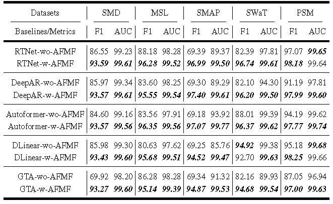
Figure 4. Results of five forecasting networks '-wo-'/'-w-' AFMF

OrigamiSL / AFMF