seaborn_objects_recipes is a Python package that extends the functionality of the Seaborn library, providing custom recipes for enhanced data visualization. This package includes below features to augment your Seaborn plots with additional capabilities.
To install seaborn_objects_recipes, run the following command:
pip install seaborn_objects_recipes- Python 3.9 or higher
- Seaborn 0.13.0 or higher
- Statsmodels 0.14.1 or higher
-
Rolling: This class provides a method to apply rolling window operations on data, enabling smooth and flexible aggregations such as moving averages.
-
LineLabel: This class facilitates the addition of labels to lines in your plots, improving readability and providing additional context directly on the graph.
-
Lowess: The Locally Weighted Scatterplot Smoothing (LOWESS) class allows for the fitting of smooth curves to data using local regression, which is particularly useful for visualizing trends in noisy datasets. It also includes options to compute confidence intervals using bootstrapping.
-
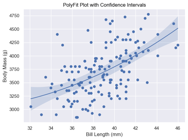
PolyFitWithCI: This class fits polynomial curves to your data and includes functionality to calculate and visualize confidence intervals, providing a robust method for polynomial regression analysis.
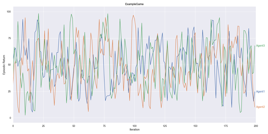
In this example, we will generate a simulated dataset and create a plot that demonstrates the use of rolling averages and line labels. The dataset simulates the performance of three agents over multiple iterations in a game. We will use the Rolling and LineLabel classes from the seaborn_objects_recipes package to enhance the visualization.
import seaborn.objects as so
import seaborn_objets_recipes as sor
import pandas as pd
import numpy as npFirst, we define a function sample_data() to generate a DataFrame with simulated data. The data includes the episodic returns of three agents over 200 iterations in a game called "ExampleGame".
def sample_data():
    # Parameters for simulation
    game = "ExampleGame"
    agents = ["Agent1", "Agent2", "Agent3"]
    num_iterations = 200
    num_agents = len(agents)

    # Create a simulated DataFrame
    np.random.seed(0)  # For reproducible results
    data = {
        "Game": [game] * num_iterations * num_agents,
        "Episodic Return": np.random.rand(num_iterations * num_agents) * 100,
        "Iteration": list(range(num_iterations)) * num_agents,
        "Agent": np.repeat(agents, num_iterations),
    }

return pd.DataFrame(data)Next, we use the seaborn.objects interface to create a plot that includes rolling averages and line labels. We utilize the Rolling class to apply a Gaussian rolling average and the LineLabel class to add informative labels to the lines.
def test_line_label():
    data = sample_data()

    (
        data.pipe(
            so.Plot, y="Episodic Return", x="Iteration", color="Agent", text="Agent"
        )
        .layout(size=(16, 8))
        .facet("Game")
        .limit(x=(0, 200))
        .scale(
            x=so.Continuous().tick(at=list(range(0, 201, 25))),
            y=so.Continuous().tick(upto=5).label(like="{x:,.0f}"),
        )
        .add(
            so.Lines(),
            so.Agg(),
            rolling := sor.Rolling(window_type="gaussian", window_kwargs={"std": 2}),
            legend=False,
        )

        .add(
            sor.LineLabel(offset=5),
            so.Agg(),
            rolling,
            legend=False,
        )
        # Display Plot
        .show()
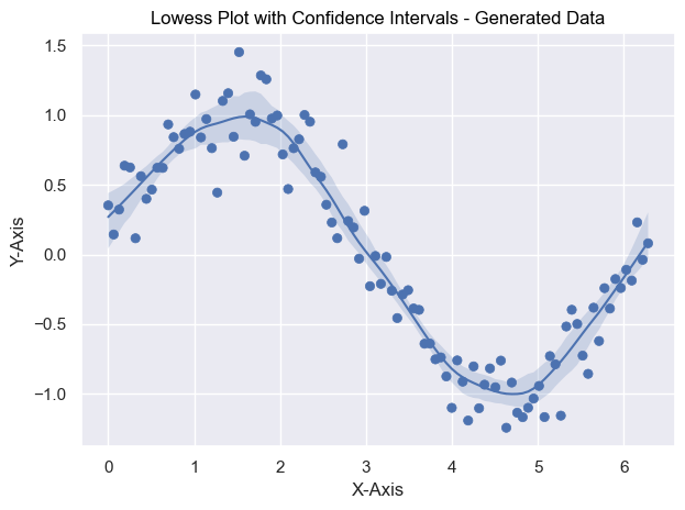
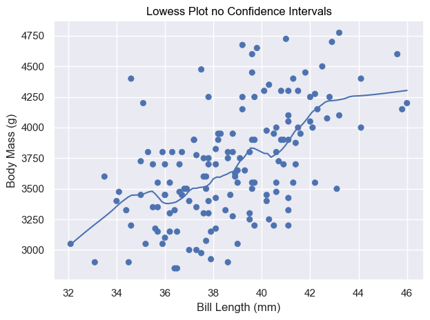
)The Lowess recipe in the seaborn_objects_recipes package provides a method for locally-weighted regression, also known as LOWESS. This technique is useful for smoothing data and visualizing trends in a dataset. LOWESS is particularly effective for non-linear data and helps in identifying patterns without assuming a specific functional form.
Key Features:
- Locally-Weighted Regression: Fit a smooth curve to your data using a local regression technique.
- Customizable Smoothing: Control the fraction of data points used for each local regression to adjust the smoothness of the curve.
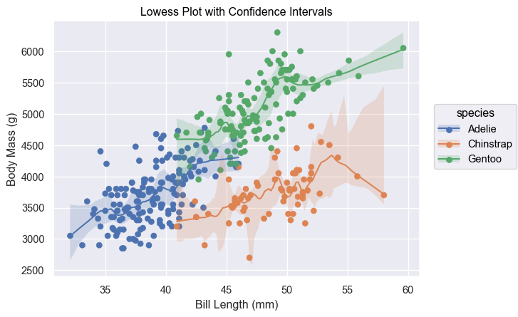
- Confidence Intervals: Optionally compute bootstrap confidence intervals to visualize the uncertainty in the smoothed curve.
Parameters:
- frac: The fraction of data used when estimating each y-value. A smaller value results in more local smoothing.
- gridsize: The number of points in the grid to which the LOWESS is applied. Higher values result in a smoother curve.
- delta: Distance within which to use linear interpolation instead of weighted regression.
- num_bootstrap: The number of bootstrap samples to use for computing confidence intervals.
- alpha: The confidence level for the intervals.
import seaborn.objects as so
import seaborn_objects_recipes as sor
import pandas as pd
import numpy as np

def test_lowess_with_ci_gen():
    # Generate data for testing
    np.random.seed(0)
    x = np.linspace(0, 2 * np.pi, 100)
    y = np.sin(x) + np.random.normal(size=100) * 0.2
    data = pd.DataFrame({"x": x, "y": y})

    # Create the plot
    plot = (
        so.Plot(data, x="x", y="y")
        .add(so.Dot())
        .add(so.Line(), lowess := sor.Lowess(frac=0.2, gridsize=100, num_bootstrap=200, alpha=0.95))
        .add(so.Band(), lowess)
        .label(x="x-axis", y="y-axis", title="Lowess Plot with Confidence Intervals - Generated Data")
    )
    # Display Plot
plot.show()import seaborn.objects as so
import seaborn as sns
import seaborn_objects_recipes as sor
def test_lowess_with_no_ci():
# Load the penguins dataset
penguins = sns.load_dataset("penguins")
# Prepare data
data = penguins.copy()
data = penguins[penguins['species'] == 'Adelie']
# Create the plot
plot = (
so.Plot(data, x="bill_length_mm", y="body_mass_g")
.add(so.Dot())
.add(so.Line(), sor.Lowess())
.label(x="Bill Length (mm)", y="Body Mass (g)", title="Lowess Plot no Confidence Intervals")
)
# Display Plot
plot.show()
import seaborn.objects as so
import seaborn as sns
import seaborn_objects_recipes as sor

def test_lowess_with_ci():

    # Load the penguins dataset
    penguins = sns.load_dataset("penguins")

    # Prepare data
    data = penguins.copy()
    data = penguins[penguins['species'] == 'Adelie']

    # Create the plot
    plot = (
        so.Plot(data, x="bill_length_mm", y="body_mass_g")
        .add(so.Dot())
        .add(so.Line(), lowess := sor.Lowess(frac=0.2, gridsize=100, num_bootstrap=200, alpha=0.95))
        .add(so.Band(), lowess)
        .label(x="Bill Length (mm)", y="Body Mass (g)", title="Lowess Plot with Confidence Intervals")
    )
    # Display Plot
    plot.show()
The PolyFitWithCI recipe in the seaborn_objects_recipes package provides a method for fitting polynomial regression models to data, including confidence intervals. Polynomial regression is useful for capturing non-linear relationships between variables, and adding confidence intervals helps visualize the uncertainty around the fitted polynomial curve.
Key Features:
- Polynomial Regression: Fit a polynomial of a specified order to your data.
- Customizable Order: Control the order of the polynomial to capture different degrees of non-linearity.
- Confidence Intervals: Compute and visualize confidence intervals around the fitted polynomial curve.
Parameters:
- order: The order of the polynomial to fit. Higher orders can capture more complex relationships but may overfit the data.
- gridsize: The number of points in the grid to which the polynomial is applied. Higher values result in a smoother curve.
- alpha: The confidence level for the intervals.
import seaborn.objects as so
import seaborn as sns
import seaborn_objects_recipes as sor

def test_polyfit_with_ci():

    # Load the penguins dataset
    penguins = sns.load_dataset("penguins")

    # Prepare data
    data = penguins.copy()
    data = data[data["species"] == "Adelie"]

    # Create the plot
    plot = (
        so.Plot(data, x="bill_length_mm", y="body_mass_g")
        .add(so.Dot())
        .add(so.Line(), PolyFitWithCI := sor.PolyFitWithCI(order=2, gridsize=100, alpha=0.05))
        .add(so.Band(), PolyFitWithCI)
        .label(x="Bill Length (mm)", y="Body Mass (g)", title="PolyFit Plot with Confidence Intervals")
    )
    # Display Plot
plot.show()Contributions are welcome! Please feel free to submit a Pull Request.
For questions or feedback regarding seaborn_objects_recipes, please contact Ofosu Osei.
-
Special thanks to @JesseFarebro for Rolling, LineLabel
-
Special thanks to @tbpassin and @kcarnold for LOWESS Smoother
