Module 5 Final Project

Repository Contest

presentation_clean.pdf - Project's Executive Summary for non-technicall audience
presentation_wComments.pptx - editable version of Executive Summary in pptx-format with speaker's thesises
student.ipynb - file with Project's code
TA_restaurants_curated.csv - analyzed dataset for the Project
eu_map.html - EU cities map for the considered dataset
Other files - (LICENSE.md, module5_project_rubric.pdf, smart.gif, README.md) - standart set of files from forked repo

Brief Description

Purpose and main files

This project was created as part of Module 5 of the Flatiron Curriculum (Data Science). The goal of the project is to build an efficient classifier using Machine Learning algorithms (not including Deep Learning algorithms). The main code implementing this task is located in student.ipynb file. Presentation with description of results and benefits for business - in the file presentation_clean.pdf.

Dataset

В качестве данных для построения модели была взята выборка из Trip Advisor, содержащая информацию о более чем 125 000 ресторанов в ЕС, которая доступна на сайте Kaggle. Dataset содержит different types of features, including:

Price Range (3 values: $ (cheap), $$-$$$ (medium), $$$$ (expensive)) - TARGET
Ranking (16k unique values)
Rating (11 unique values)
Number of Reviews (2k unique values)
City (31 unique values)
Cuisine (125 types of cuisine style in individual combination (list) for each sample)
ID_TA (ID-type for restaurant)
URL_TA (URL - specific for restaurant)
Reviews (collection of text comments for each sample)

Business goals

The Price Range indicator that has 3 classes was selected as a target. This is due to the fact that understanding the price range of a restaurant depending on factors such as the city, type of cuisine, etc., is beneficial for investors in this sector. In order to plan investments in the purchase of an existing restaurant or the creation of a new one, it is necessary to build a financial model (or financial forecast), where the key factors are the revenue determined by the level of occupancy of the restaurant and prices. If there is no explicit information on the level of occupancy in this database, then the price range is exactly what can be studied.

Thus, the attempt to build a price range classifier undertaken in this project may be useful for the corresponding business metrics.

Description of data and some statistics

Unrelevant features and Dataset after Cleaning

In further analysis, I have excluded a number of features that either do not provide useful information or are of little use given the methodology adopted in the project. The most significant here is the exclusion of NLP algorithms and most likely neural networks, which is not foreseen in this project.
Also, it's important to note that about 38% of the price range data was missing, so I left only 78 thousand observations for analysis. The visual diagram of Target distribution by classes is presented below. Also categorical data by city and by cuisine style were encoded by One-Hot-Encoder. Total size of the dataset: 77 672 samples : 159 features.

Location

Restaurant Dataset covers almost all major EU cities except for some Eastern European cities and is a representative of the industry in the region.

Data Preprocessing and Model construction

Data Preprocessing and EDA

As part of the analysis, joint KDE, the correlation matrix and the cluster analysis were reviewed. Despite the fact that it visually seems that some values can form clusters (such as Rating and Ranking - for 2D-KDE), Silhouette Score using the KMeans model is estimated at 0.04 (for 3 clusters).
Additionally, clusters by DBSCAN were evaluated for different hyperparameter configurations: the absolute value of Silhouette Score metric did not exceed 0.25. So no significant clusters revealed here.

To reduce the dimension of the feature space and exclude the correlated features, the PCA method was applied to the data with a selected number of components - 87 (from the original 159), preserving 97.5% of the Variation.
Scaling of data was performed 2 times: before PCA and after PCA by MinMaxScaler.

Preparements for Modelling

Since the search for the optimal model and optimal hyperparameters is an iterative and repetitive process, a special class was written to facilitate and reduce the amount of code: Single_Model, which is essentially a wrapper for GridSearchCV, automatically starts the learning process when initializing an instance, and also includes a number of methods for quick output of results and objects.

best_model() - returns best model
show_grid_result() - print short report with metrics (accuracy on train and test sets) and best hyperparams
best_params() - returns best hyperparams in dict
best_score() - return best score
best_model() - return best_model

With this in mind, the calculation of the parameter search is quite concise, as in the example below:

xgb_grid = {'booster': ['gbtree'], 
            'n_estimators': [100],
            'learning_rate': [0.1],
            'max_depth': [7]}
xgb_gridmodel = Single_Model(xgb, X_train_pca, y_train, cv=4, param_grid=xgb_grid)
xgb_gridmodel.show_grid_results()
xgb_best_model = xgb_gridmodel.best_model()

Applied ML Algorythms and Accuracy results

With the exception of XG-Boost, all algorithms used in the project are available in the Scikit-Learn library.
The values in brackets are for validation and train folds with best hyperparameters.

K-Nearest Neighbors (0.738-0.775)
Decision Tree (0.730-0.739)
Support Vector Machine (0.743-0.744)
Logistic Regression (0.746-0.746)
Multinomial Bayes Classifier (0.701-0.701)
Random Forest (0.742-0.771)
ADA-Boosting (0.738-0.742)
XG-Boost (0.743-0.749)

Models ranking and Monte-Carlo Simulation

After selecting hyperparameters, I retrained all classes of models on the full TRAINSET (with the selection of the optimal number of PCA), the final choice was the XG-Boost algorithm with the following metrics:

accuracy score on TEST SET = 0.75
accuracy score on TRAIN SET = 0.80

Corresponding confusion matrix

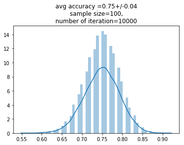
As part of my research curiosity I additionally tested the model for accuracy by feeding small bootstrap-samples (with n=100) 10k-times from TEST DATASET and combined (TEST+TRAIN) DATASET. The results of the trained model showed relative stability of accuracy:

for TEST: mean = 0.75, std = 0.04
for TEST+TRAIN: mean = 0.79, std = 0.04 An example of the corresponding histogram is presented below.

Future Work

The research of such dataset can be used for different purposes. In particular, instead of PriceRange it is possible to study the influence of factors on Rating (11-classes variable), which is of interest for a marketing research and can (implicitly) reflect the second component of Revenue - demand. With this formulation of the task, it is of particular importance to study and implement text data of the Reviews variable, processing of which is most likely to be convenient with the help of full-dense perseptrons (TF-IDF model) or recursive neural networks.

NuranKZ / dsc-mod-5-project-online-ds-sp-000