
We implemented a multi-class classification approach for disaster assessment from the given data set of post earthquake satellite imagery. The idea was to classify the different damage types in an image.
- Introduction
- File-Structure
- Getting Started
- Usage
- Theory
- Future-Work
- Trouble-Shooting
- Contributors
- Results
- Acknowledgements and Resources
We need to extract data from the post earthquake imagery training set and classify buildings on the basis of how damaged they are. The buildings are classified into 5 types .i.e:
- Destroyed buildings
- Major Damaged buildings
- Minor Damaged buildings
- No damaged buildings
- Unclassified

📦Vision-Beyond-Limits-main
 ┣ 📂Mask-20211120T183800Z-001
 ┃ ┗ 📂Mask
 ┃ ┃ ┣ 📜mexico-earthquake_00000001_post_disaster.png
 ┃ ┃ ┣ 📜mexico-earthquake_00000002_post_disaster.png
 ┃ ┃ ┣ 📜mexico-earthquake_00000003_post_disaster.png
 ┃ ┃ ┣ 📜mexico-earthquake_00000004_post_disaster.png
 ┃ ┃ ┣ 📜mexico-earthquake_00000007_post_disaster.png
 ┃ ┃ ┗ ...
 ┣ 📂Output_classified_images
 ┃ ┣ 📜Output_1.png
 ┃ ┣ 📜Output_10.png
 ┃ ┣ 📜Output_11.png
 ┃ ┣ 📜Output_12.png
 ┃ ┗ ...
 ┣ 📂vbl_data
 ┃ ┣ 📂augmented_data
 ┃ ┃ ┣ 📂data_180
 ┃ ┃ ┃ ┣ 📂images_180
 ┃ ┃ ┃ ┃ ┣ 📜mexico-earthquake_00000001_post_disaster.png_180.png
 ┃ ┃ ┃ ┃ ┣ 📜mexico-earthquake_00000002_post_disaster.png_180.png
 ┃ ┃ ┃ ┃ ┣ 📜mexico-earthquake_00000003_post_disaster.png_180.png
 ┃ ┃ ┃ ┃ ┣ 📜mexico-earthquake_00000004_post_disaster.png_180.png
 ┃ ┃ ┃ ┃ ┣ 📜mexico-earthquake_00000007_post_disaster.png_180.png
 ┃ ┃ ┃ ┃ ┗ ...
 ┃ ┃ ┃ ┗ 📂masks_180
 ┃ ┃ ┃ ┃ ┣ 📜mexico-earthquake_00000001_post_disaster.png_180.png
 ┃ ┃ ┃ ┃ ┣ 📜mexico-earthquake_00000002_post_disaster.png_180.png
 ┃ ┃ ┃ ┃ ┣ 📜mexico-earthquake_00000003_post_disaster.png_180.png
 ┃ ┃ ┃ ┃ ┣ 📜mexico-earthquake_00000004_post_disaster.png_180.png
 ┃ ┃ ┃ ┃ ┣ 📜mexico-earthquake_00000007_post_disaster.png_180.png
 ┃ ┃ ┃ ┃ ┗ ...
 ┃ ┃ ┣ 📂data_270
 ┃ ┃ ┃ ┣ 📂images_270
 ┃ ┃ ┃ ┃ ┣ 📜mexico-earthquake_00000001_post_disaster.png_270.png
 ┃ ┃ ┃ ┃ ┣ 📜mexico-earthquake_00000002_post_disaster.png_270.png
 ┃ ┃ ┃ ┃ ┣ 📜mexico-earthquake_00000003_post_disaster.png_270.png
 ┃ ┃ ┃ ┃ ┣ 📜mexico-earthquake_00000004_post_disaster.png_270.png
 ┃ ┃ ┃ ┃ ┣ 📜mexico-earthquake_00000007_post_disaster.png_270.png
 ┃ ┃ ┃ ┃ ┗ ...
 ┃ ┃ ┃ ┗ 📂masks_270
 ┃ ┃ ┃ ┃ ┣ 📜mexico-earthquake_00000001_post_disaster.png_270.png
 ┃ ┃ ┃ ┃ ┣ 📜mexico-earthquake_00000002_post_disaster.png_270.png
 ┃ ┃ ┃ ┃ ┣ 📜mexico-earthquake_00000003_post_disaster.png_270.png
 ┃ ┃ ┃ ┃ ┣ 📜mexico-earthquake_00000004_post_disaster.png_270.png
 ┃ ┃ ┃ ┃ ┣ 📜mexico-earthquake_00000007_post_disaster.png_270.png
 ┃ ┃ ┃ ┃ ┗ ...
 ┃ ┃ ┗ 📂data_90
 ┃ ┃ ┃ ┣ 📂images_90
 ┃ ┃ ┃ ┃ ┣ 📜mexico-earthquake_00000001_post_disaster.png_90.png
 ┃ ┃ ┃ ┃ ┣ 📜mexico-earthquake_00000002_post_disaster.png_90.png
 ┃ ┃ ┃ ┃ ┣ 📜mexico-earthquake_00000003_post_disaster.png_90.png
 ┃ ┃ ┃ ┃ ┣ 📜mexico-earthquake_00000004_post_disaster.png_90.png
 ┃ ┃ ┃ ┃ ┣ 📜mexico-earthquake_00000007_post_disaster.png_90.png
 ┃ ┃ ┃ ┃ ┗ ...
 ┃ ┃ ┃ ┗ 📂masks_90
 ┃ ┃ ┃ ┃ ┣ 📜mexico-earthquake_00000001_post_disaster.png_90.png
 ┃ ┃ ┃ ┃ ┣ 📜mexico-earthquake_00000002_post_disaster.png_90.png
 ┃ ┃ ┃ ┃ ┣ 📜mexico-earthquake_00000003_post_disaster.png_90.png
 ┃ ┃ ┃ ┃ ┣ 📜mexico-earthquake_00000004_post_disaster.png_90.png
 ┃ ┃ ┃ ┃ ┣ 📜mexico-earthquake_00000007_post_disaster.png_90.png
 ┃ ┃ ┃ ┃ ┗ ...
 ┃ ┣ 📂orginal_images
 ┃ ┃ ┣ 📜mexico-earthquake_00000001_post_disaster.png
 ┃ ┃ ┣ 📜mexico-earthquake_00000002_post_disaster.png
 ┃ ┃ ┣ 📜mexico-earthquake_00000003_post_disaster.png
 ┃ ┃ ┣ 📜mexico-earthquake_00000004_post_disaster.png
 ┃ ┃ ┣ 📜mexico-earthquake_00000007_post_disaster.png
 ┃ ┃ ┗ ...
 ┃ ┗ 📂original_mask
 ┃ ┃ ┣ 📜mexico-earthquake_00000001_post_disaster.png
 ┃ ┃ ┣ 📜mexico-earthquake_00000002_post_disaster.png
 ┃ ┃ ┣ 📜mexico-earthquake_00000003_post_disaster.png
 ┃ ┃ ┣ 📜mexico-earthquake_00000004_post_disaster.png
 ┃ ┃ ┣ 📜mexico-earthquake_00000007_post_disaster.png
 ┃ ┃ ┗ ...
 ┣ 📜augment.py
 ┣ 📜LICENSE
 ┣ 📜masking.py
 ┣ 📜Model.ipynb
 ┣ 📜README.md
 ┗ 📜README.txt
The following modules or packages/environment are required for running the code
-
Python v3 is required
-
Libraries like Keras and tensorflow are also required for machine learning algorithms
-
Numpy and OpenCV are 2 very important libraries for image processing
-
Matplotlib is used to plot graphs of accuracy and loss
-
Sklearn library is used for encoding the images and providing the classes with labels
Install:
pip install -r requirements.txt
-
Clone the repo
git clone https://github.com/Neel-Shah-29/Vision-Beyond-Limits.git
Before you start, you need to have two directories: Images(containing .png file) and Labels(containing .json file).
To augment data you can run
augment.py, it will save images rotated by 90°, 180° and 270°.
cd /path/to/Vision-Beyond-Limits/
python3 masking.py
Modify correct path of Images(containg .png), Label(containg .json) and Mask where masked images wil be stored in ths code.
Open vbl.ipynb and run all cells in sequencial order.
Enter paths of images and masked images wherever specified.
Good performance of deep learning algorithms is limited to the size of data available, and the network structure is considered. One of the most critical challenges for using a deep learning method for monitoring the buildings damaged in the disaster is that the training images of damaged targets are usually not very much. So models that can give considerably high accuracy compared to that of a regular model on a small dataset needed to be chosen.

- Convolutional layer
- Pooling layer
- Fully-connected (FC) layer
The convolutional layer is the first layer of a convolutional network. While convolutional layers can be followed by additional convolutional layers or pooling layers, the fully-connected layer is the final layer. With each layer, the CNN increases in its complexity, identifying greater portions of the image. Earlier layers focus on simple features, such as colors and edges. As the image data progresses through the layers of the CNN, it starts to recognize larger elements or shapes of the object until it finally identifies the intended object. We have used U-Net model which is convolutional network architecture for fast and precise segmentation of images.

When we solve a classification problem having only two class labels, then it becomes easy for us to filter the data, apply any classification algorithm, train the model with filtered data, and predict the outcomes. But when we have more than two class instances in input train data, then it might get complex to analyze the data, train the model, and predict relatively accurate results. To handle these multiple class instances, we use multi-class classification. Multi-class classification is the classification technique that allows us to categorize the test data into multiple class labels present in trained data as a model prediction.There are mainly two types of multi-class classification techniques:-
- One vs. All (one-vs-rest)
- One vs. One


Adam optimizer involves a combination of two gradient descent methodologies:
- Momentum:
This algorithm is used to accelerate the gradient descent algorithm by taking into consideration the ‘exponentially weighted average’ of the gradients. Using averages makes the algorithm converge towards the minima in a faster pace.
- Root Mean Square Propagation (RMSP):
Root mean square prop or RMSprop is an adaptive learning algorithm that tries to improve AdaGrad. Instead of taking the cumulative sum of squared gradients like in AdaGrad, it takes the ‘exponential moving average’. Adam Optimizer inherits the strengths or the positive attributes of the above two methods and builds upon them to give a more optimized gradient descent.

- Focal Loss: By using Focal Loss we can reduce the imbalance in the dataset. We have tried focal loss as a loss function in our problem as the classes were highly imbalanced, focal loss can be useful in such cases.

- Categorical_crossentropy: Categorical cross entropy is a loss function that is used in multi-class classification tasks. These are tasks where an example can only belohttps://user-images.githubusercontent.com/84740927/147950518-d6b03f7a-56e2-41f2-9032-e39e9f45f20c.pngng to one out of many possible categories, and the model must decide which one.Our problem was on a similar basis so we tried it.

We tired solving this problems in 5 steps:
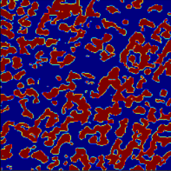
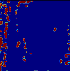
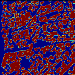
- Get mask
First we need to get mask ready. To do that, we have used skimage and matplotlib libraires on our JSON data to from multi-label masking which will used for traing the model for damage detection.
- Define model
We defined Unet model which takes n_classes, IMG_HEIGHT, IMG_WIDTH, IMG_CHANNELS as argument. We have used softmax as activation function as in our case its multi-class classification.
- Encode data
Now we will encode our labels using LabelEncoder from sklearn. Encoder add values from 0-5 (as we have 6 classes) to our label. Further split our data set into train image and test image in 9:1 ratio.
- Train model
Next, we complied the model using Adam , optimizer, focal-loss as loss function and accuracy metric and used sample weights as data was imbalanced. We tried different things while training the model like changing the number of epochs , changing the weights that we have defined , also we have changed the image size to see if there is any change in the accuracy or not.
- Test model
After training the model we saved the model to use it while testing. Finally we are ready to test our model, plot accuracy and loss graph and get our values of IoU, Precison and Recall. You can check the results that we got in Results section.
- FlowChart

- We would like to improve accuracy of our model and test our model on bigger datasets.
- We can use better approaches to handle skewed data set.
- We can use Data loader to train our model on more no of epochs.
- While working on google colab we faced many errors due to tensorflow versions, solution to this would be to see the requirements of model properly and accordingly install the required versions.
- While defining class weights it should be converted into a dictionary with your labels as key and associated weight as value to avoid any errors.
- Other errors were solved with help of google.