receptivefield

Gradient based receptive field estimation for Convolutional Neural Networks. receptivefield uses backpropagation of the gradients from output feature map to input image in order to estimate the size (width, height), stride and offset of resulting receptive field. Numerical estimation of receptive field can be useful when dealing with more complicated neural networks like ResNet, Inception (see notebooks) where analytical approach of computing receptive fields cannot be used.

Installation

Requires: python (in version >= 3.6), keras, tensorflow, numpy, matplotlib, pillow (check requirements.txt)
pip install receptivefield

Some remarks

In order to get better results or even avoid NaNs in the estimated receptive field parameters, it is suggested to use Linear (instead Relu) activation and AvgPool2D instead of MaxPool2D. This improves gradient flow in the network and hence better signal in the input image. Note, that this is required only for RF estimation.
Additionally, one may even initialize network with constant positive values in all weights (positive if max pooling is used) and set biases to zero. In case of Keras API this can be obtained by setting init_weight=True in the KerasReceptiveField(init_weight=True) constructor.

Limitations

Numerical approach cannot be used when RF is larger that input image, however one may try to increase the input image size, sice RF parameters depend on the architecture not image.

Supported APIs

Currently only Keras and Tensorflow API are supported. However it should be possible to extend receptivefield functionality by deriving abstract class ReceptiveField in base.py file.

Keras with KerasReceptiveField, example usage in notebooks/keras_api.ipynb
Tensorflow with TFReceptiveField example usage in notebooks/tensorflow_api.ipynb

How does it work?

Define build_function which returns Keras model

def model_build_func(input_shape=[224, 224, 3]):
    ...
    return Model(input, output)

Compute receptive field parameters with KerasReceptiveField

from receptivefield.keras import KerasReceptiveField
rf_params = KerasReceptiveField(model_build_func).compute(
    input_shape=[224, 224, 3], # this will be passed to model_build_func
    input_layer='input_image', # must exist - usually input image layer
    output_layer='feature_map' # for example last conv layer
)

The rf_params is object of class ReceptiveFieldDescription e.g.
```
ReceptiveFieldDescription(
        offset=(17.0, 17.0), 
        stride=(4.0, 4.0), 
        size=Size(w=34, h=34)
)
```
- offset - defines location of the first left-top anchor in the image coordinates (defined in pixels).
- stride - defines how much RF of the network moves w.r.t unit displacement in the feature_map tensor.
- size - defines the effective area in the input image which one point in the feature_map tensor is seeing.

Keras minimal - copy/paste example

Python code:

from keras.layers import Conv2D, Input, AvgPool2D
from keras.models import Model
from receptivefield.image import get_default_image
from receptivefield.keras import KerasReceptiveField

# define model function
def model_build_func(input_shape):
    act = 'linear' # see Remarks
    inp = Input(shape=input_shape, name='input_image')
    x = Conv2D(32, (7, 7), activation=act)(inp)
    x = Conv2D(32, (5, 5), activation=act)(x)
    x = AvgPool2D()(x)
    x = Conv2D(64, (5, 5), activation=act, name='feature_grid')(x)
    x = AvgPool2D()(x)
    model = Model(inp, x)
    return model

shape = [64, 64, 3]
# compute receptive field
rf = KerasReceptiveField(model_build_func, init_weights=True)
rf_params = rf.compute(shape, 'input_image', 'feature_grid')
# debug receptive field
rf.plot_rf_grid(get_default_image(shape, name='doge'))

Logger output + example RF grid

Using TensorFlow backend.
[2017-11-28 21:47:14,327][ INFO][keras.py]::Feature map shape: (None, 23, 23, 64)
[2017-11-28 21:47:14,328][ INFO][keras.py]::Input shape      : (None, 64, 64, 3)
[2017-11-28 21:47:14,471][DEBUG][base.py]::Computing RF at center (11, 11) with offset GridPoint(x=0, y=0)
[2017-11-28 21:47:14,676][DEBUG][base.py]::Computing RF at center (11, 11) with offset GridPoint(x=1, y=1)
[2017-11-28 21:47:14,779][DEBUG][base.py]::Estimated RF params: ReceptiveFieldDescription(offset=(10.0, 10.0), stride=(2.0, 2.0), size=Size(w=20, h=20))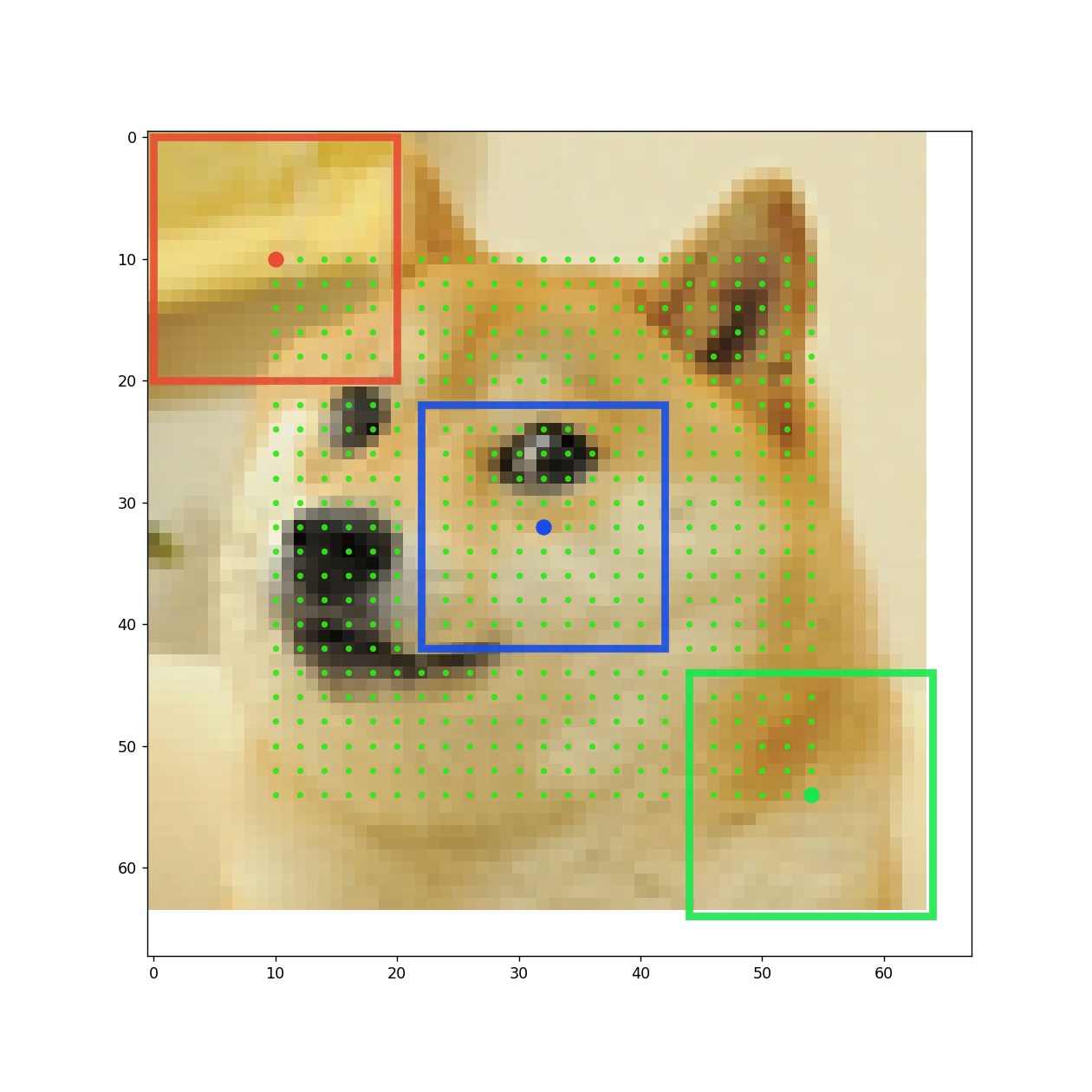

Keras more detailed example

Here we show, how to estimate effective receptive field of any Keras model.

Create model build_function which returns model. This function should accept one parameter input_shape.

from keras.layers import Conv2D, Input
from keras.layers import AvgPool2D
from keras.models import Model

def model_build_func(input_shape):
    activation = 'linear'
    padding='valid'
    
    inp = Input(shape=input_shape, name='input_image')
    x = Conv2D(32, (5, 5), padding=padding, activation=activation)(inp)
    x = Conv2D(32, (3, 3), padding=padding, activation=activation)(x)
    x = AvgPool2D()(x)
    x = Conv2D(64, (3, 3), activation=activation, padding=padding)(x)
    x = Conv2D(64, (3, 3), activation=activation, padding=padding)(x)
    x = AvgPool2D()(x)
    x = Conv2D(128, (3, 3), activation=activation, padding=padding)(x)
    x = Conv2D(128, (3, 3), activation=activation, padding=padding, name='feature_grid')(x)

    model = Model(inp, x)
    return model

Check if model is building properly:

model = model_build_func(input_shape=(96, 96, 3))
model.summary()

_________________________________________________________________
Layer (type)                 Output Shape              Param #   
=================================================================
input_image (InputLayer)     (None, 96, 96, 3)         0         
_________________________________________________________________
conv2d_1 (Conv2D)            (None, 92, 92, 32)        2432      
_________________________________________________________________
conv2d_2 (Conv2D)            (None, 90, 90, 32)        9248      
_________________________________________________________________
average_pooling2d_1 (Average (None, 45, 45, 32)        0         
_________________________________________________________________
conv2d_3 (Conv2D)            (None, 43, 43, 64)        18496     
_________________________________________________________________
conv2d_4 (Conv2D)            (None, 41, 41, 64)        36928     
_________________________________________________________________
average_pooling2d_2 (Average (None, 20, 20, 64)        0         
_________________________________________________________________
conv2d_5 (Conv2D)            (None, 18, 18, 128)       73856     
_________________________________________________________________
feature_grid (Conv2D)        (None, 16, 16, 128)       147584    
=================================================================
Total params: 288,544
Trainable params: 288,544
Non-trainable params: 0

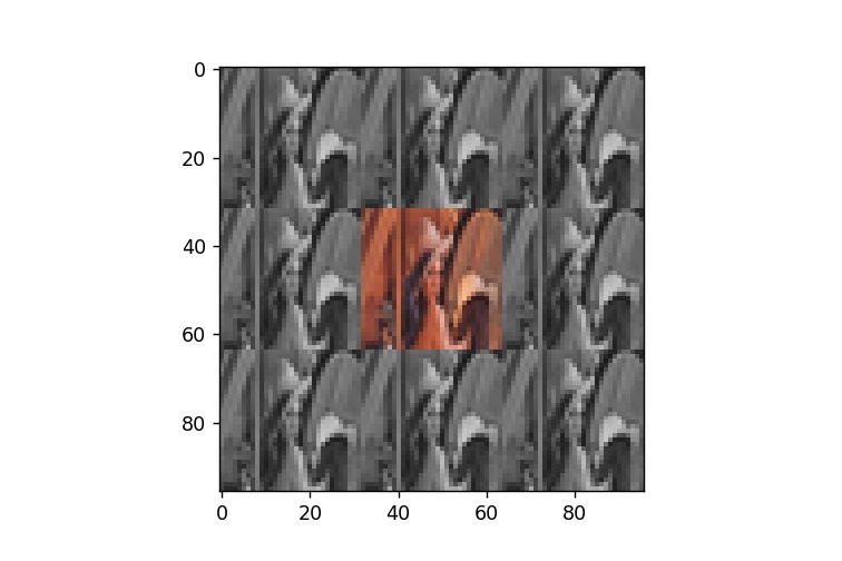
This step is not required but it is useful to plot results in the example image. For instance you would like to see what is the size of network receptive field in comparision to some objects you wish detect (or localize) by this network.
```
from receptivefield.image import get_default_image
import matplotlib.pyplot as plt
# Load sample image of `Lena`.
image = get_default_image(shape=(32, 32), tile_factor=1)
plt.imshow(image)
```

Compute receptive field of the network by calling rf.compute

from receptivefield.keras import KerasReceptiveField

rf = KerasReceptiveField(model_build_func, init_weights=False)

rf_params = rf.compute(
    input_shape=image.shape, 
    input_layer='input_image', 
    output_layer='feature_grid'
)
print(rf_params)

The resulting receptive field is:

ReceptiveFieldDescription(
        offset=(17.0, 17.0), 
        stride=(4.0, 4.0), 
        size=Size(w=34, h=34)
)

Input shape: rf.input_shape==GridShape(n=None, w=96, h=96, c=3)
Output feature map shape: rf.output_shape==GridShape(n=None, w=16, h=16, c=1). Note, that number of channels in the output feature map is set to 1 but this is used internally by receptivefield.
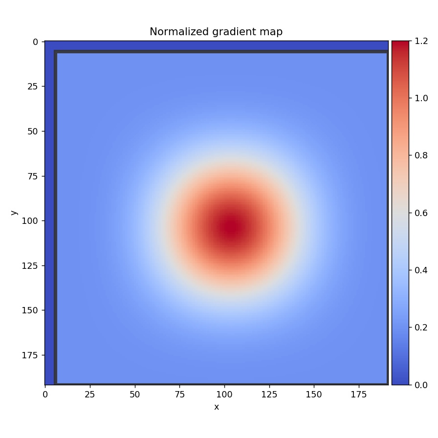
You may want to see how gradients backpropagate to the input image. Here point=(8, 8) refers to the (W, H) position of the source signal from the output grid.
```
rf.plot_gradient_at(point=(8, 8), image=None, figsize=(7, 7))
```

Or even plot whole receptive field grid:

rf.plot_rf_grid(custom_image=image, figsize=(6, 6))

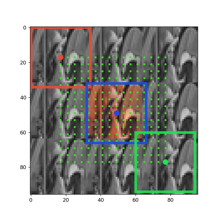
In the above, the red rectangle corresponds to the area which top-left grid point is seeing in the input image. Blue rectangle corresponds to the central grid point, green to the bottom-right point. Green dots show the position of the centers of the grid anchors in the source image.

Naruto-Sasuke / receptivefield