
This project uses a simulated Kuka KR210 6 degree of freedom robotic arm to pick up a cylinder placed on a shelf and drop it in a bucket nearby.
The cylinder position can be generated in different positions each time. Inverse kinematics were used to calculate the joint angles necessary to move the Kuka arm from the starting position to placing the gripper around the cylinder and then placing the cylinder into the bin.
Here is a Denavit-Hartenberg (DH) diagram of the Kuka KR210 courtesy of Udacity:

The arm consists of six revolute joints connected in linear fashion.
Based on the arm's specifications, the following parameter were derived:
| n | theta | d | a | alpha |
|---|---|---|---|---|
| 0 | - | - | 0 | 0 |
| 1 | theta1 | 0.75 | 0.35 | -pi/2 |
| 2 | theta2 | 0 | 1.25 | 0 |
| 3 | theta3 | 0 | -0.054 | -pi/2 |
| 4 | theta4 | 1.5 | 0 | pi/2 |
| 5 | theta5 | 0 | 0 | -pi/2 |
| 6 | theta6 | 0.303 | 0 | 0 |
The a and alpha parameters do not change because they are specific to each arm. However, the theta and d parameters can change depending on the orientation of the arm. But for this arm, only the theta parameters will change since all the joints are revolute.
All of the joints have their own transformation matrix that describes their position and orientation relative to prior joints.
The transformation matrix can be calculated by substituting the DH parameters from the table above into this matrix using this TF_Matrix function for convenience:
def TF_Matrix(alpha, a, d, q):
    TF = Matrix([[cos(q), -sin(q), 0, a],
     [sin(q)*cos(alpha), cos(q)*cos(alpha), -sin(alpha), -sin(alpha)*d],
     [sin(q)* sin(alpha), cos(q)*sin(alpha), cos(alpha), cos(alpha)*d],
     [0,0,0,1]])
    return TF
The .subs convenience method for matrices in Sympy was used to create the transformation matrices for each joint like so:
  T0_1 = TF_Matrix(alpha0, a0, d1, q1).subs(DH_Table)
  T1_2 = TF_Matrix(alpha1, a1, d2, q2).subs(DH_Table)
  T2_3 = TF_Matrix(alpha2, a2, d3, q3).subs(DH_Table)
  T3_4 = TF_Matrix(alpha3, a3, d4, q4).subs(DH_Table)
  T4_5 = TF_Matrix(alpha4, a4, d5, q5).subs(DH_Table)
  T5_6 = TF_Matrix(alpha5, a5, d6, q6).subs(DH_Table)
  T6_EE = TF_Matrix(alpha6, a6, d7, q7).subs(DH_Table)
The transformation matrices for each joint are thus:
Joint 1 T0_1:
[[cos(q1), -sin(q1), 0, 0],
[sin(q1), cos(q1), 0, 0],
[0, 0, 1, 0.750000000000000],
[0, 0, 0, 1]]
Joint 2 T1_2:
[[cos(q2 - 0.5*pi), -sin(q2 - 0.5*pi), 0, 0.350000000000000],
[0, 0, 1, 0],
[-sin(q2 - 0.5*pi), -cos(q2 - 0.5*pi), 0, 0],
[0, 0, 0, 1]]
Joint 3 T2_3:
[[cos(q3), -sin(q3), 0, 1.25000000000000],
[sin(q3), cos(q3), 0, 0],
[0, 0, 1, 0],
[0, 0, 0, 1]]
Joint 4 T3_4:
[[cos(q4), -sin(q4), 0, -0.0540000000000000],
[0, 0, 1, 1.50000000000000],
[-sin(q4), -cos(q4), 0, 0],
[0, 0, 0, 1]]
Joint 5 T4_5
[[cos(q5), -sin(q5), 0, 0],
[0, 0, -1, 0],
[sin(q5), cos(q5), 0, 0],
[0, 0, 0, 1]]
Joint 6 T5_6
[[cos(q6), -sin(q6), 0, 0],
[0, 0, 1, 0],
[-sin(q6), -cos(q6), 0, 0],
[0, 0, 0, 1]]
Joint 7 (End Effector) T6_EE
[[1, 0, 0, a6],
[0, 1, 0, 0],
[0, 0, 1, 0.303000000000000],
[0, 0, 0, 1]]
The full transformation for the arm is thus:
T0_EE = simplify(T0_1 * T1_2 * T2_3 * T3_4 * T4_5 * T5_6 * T6_EE)
Which results in the matrix:
[[((sin(q1)*sin(q4) + sin(q2 + q3)*cos(q1)*cos(q4))*cos(q5) + sin(q5)*cos(q1)*cos(q2 + q3))*cos(q6) + (sin(q1)*cos(q4) - sin(q4)*sin(q2 + q3)*cos(q1))*sin(q6), -((sin(q1)*sin(q4) + sin(q2 + q3)*cos(q1)*cos(q4))*cos(q5) + sin(q5)*cos(q1)*cos(q2 + q3))*sin(q6) + (sin(q1)*cos(q4) - sin(q4)*sin(q2 + q3)*cos(q1))*cos(q6), -(sin(q1)*sin(q4) + sin(q2 + q3)*cos(q1)*cos(q4))*sin(q5) + cos(q1)*cos(q5)*cos(q2 + q3), 1.0*a6*sin(q1)*sin(q4)*cos(q5)*cos(q6) + 1.0*a6*sin(q1)*sin(q6)*cos(q4) - 1.0*a6*sin(q4)*sin(q6)*sin(q2 + q3)*cos(q1) + 1.0*a6*sin(q5)*cos(q1)*cos(q6)*cos(q2 + q3) + 1.0*a6*sin(q2 + q3)*cos(q1)*cos(q4)*cos(q5)*cos(q6) - 0.303*sin(q1)*sin(q4)*sin(q5) + 1.25*sin(q2)*cos(q1) - 0.303*sin(q5)*sin(q2 + q3)*cos(q1)*cos(q4) - 0.054*sin(q2 + q3)*cos(q1) + 0.303*cos(q1)*cos(q5)*cos(q2 + q3) + 1.5*cos(q1)*cos(q2 + q3) + 0.35*cos(q1)], [((sin(q1)*sin(q2 + q3)*cos(q4) - sin(q4)*cos(q1))*cos(q5) + sin(q1)*sin(q5)*cos(q2 + q3))*cos(q6) - (sin(q1)*sin(q4)*sin(q2 + q3) + cos(q1)*cos(q4))*sin(q6), ((-sin(q1)*sin(q2 + q3)*cos(q4) + sin(q4)*cos(q1))*cos(q5) - sin(q1)*sin(q5)*cos(q2 + q3))*sin(q6) - (sin(q1)*sin(q4)*sin(q2 + q3) + cos(q1)*cos(q4))*cos(q6), (-sin(q1)*sin(q2 + q3)*cos(q4) + sin(q4)*cos(q1))*sin(q5) + sin(q1)*cos(q5)*cos(q2 + q3), -1.0*a6*sin(q1)*sin(q4)*sin(q6)*sin(q2 + q3) + 1.0*a6*sin(q1)*sin(q5)*cos(q6)*cos(q2 + q3) + 1.0*a6*sin(q1)*sin(q2 + q3)*cos(q4)*cos(q5)*cos(q6) - 1.0*a6*sin(q4)*cos(q1)*cos(q5)*cos(q6) - 1.0*a6*sin(q6)*cos(q1)*cos(q4) + 1.25*sin(q1)*sin(q2) - 0.303*sin(q1)*sin(q5)*sin(q2 + q3)*cos(q4) - 0.054*sin(q1)*sin(q2 + q3) + 0.303*sin(q1)*cos(q5)*cos(q2 + q3) + 1.5*sin(q1)*cos(q2 + q3) + 0.35*sin(q1) + 0.303*sin(q4)*sin(q5)*cos(q1)], [(-sin(q5)*sin(q2 + q3) + cos(q4)*cos(q5)*cos(q2 + q3))*cos(q6) - sin(q4)*sin(q6)*cos(q2 + q3), (sin(q5)*sin(q2 + q3) - cos(q4)*cos(q5)*cos(q2 + q3))*sin(q6) - sin(q4)*cos(q6)*cos(q2 + q3), -sin(q5)*cos(q4)*cos(q2 + q3) - sin(q2 + q3)*cos(q5), -1.0*a6*sin(q4)*sin(q6)*cos(q2 + q3) - 1.0*a6*sin(q5)*sin(q2 + q3)*cos(q6) + 1.0*a6*cos(q4)*cos(q5)*cos(q6)*cos(q2 + q3) - 0.303*sin(q5)*cos(q4)*cos(q2 + q3) - 0.303*sin(q2 + q3)*cos(q5) - 1.5*sin(q2 + q3) + 1.25*cos(q2) - 0.054*cos(q2 + q3) + 0.75], [0, 0, 0, 1]]
If we substitute zero for all thetas, we get a matrix representing the origin position of the Kuka Arm:
[[0, 0, 1, 2.15300000000000],
[0, -1, 0, 0],
[1, 0, 0, 1.94600000000000],
[0, 0, 0, 1]]


The following code was used to calculate the inverse kinematics:
theta1 = atan2(WC[1], WC[0]) #inferred from the position of the end effector

side_a = 1.501
side_b = sqrt(pow(sqrt(WC[0] * WC[0] + WC[1] * WC[1]) - 0.35, 2)+ pow((WC[2] - 0.75), 2))
side_c = 1.25

angle_a = acos((side_b * side_b + side_c * side_c - side_a * side_a) / (2 * side_b * side_c))
angle_b = acos((side_a * side_a + side_c * side_c - side_b * side_b) / (2 * side_a * side_c))
angle_c = acos((side_a * side_a + side_b * side_b - side_c * side_c ) / (2 * side_a * side_b))

theta2 = pi/2. - angle_a - atan2(WC[2] - 0.75, sqrt(WC[0] + WC[1] * WC[1]) - 0.35)
theta3 = pi/2. - (angle_b + 0.036) # 0.036 accounts for sag in link4 of -0.054m


R0_3 = T0_1[0:3,0:3] * T1_2[0:3,0:3] * T2_3[0:3,0:3]
R0_3 = R0_3.evalf(subs={q1: theta1, q2:theta2, q3: theta3})

# The inverse of the rotation matrix is the transpose as it is an orthogonal matrix
# This saves on compute time

R3_6 = R0_3.transpose() * ROT_EE

# Euler angles from rotation matrix

theta4 = atan2(R3_6[2,2], -R3_6[0,2])
theta5 = atan2(sqrt(R3_6[0,2]*R3_6[0,2] + R3_6[2,2] * R3_6[2,2]), R3_6[1,2])
theta6 = atan2(-R3_6[1,1], R3_6[1,0])
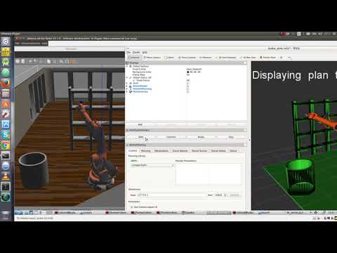
Successful Pick and Place using the IK_server.py code:

A successful pick and place operation is posted on youtube here:
To run projects from this repository you need version 7.7.0+ If your gazebo version is not 7.7.0+, perform the update as follows:
$ sudo sh -c 'echo "deb http://packages.osrfoundation.org/gazebo/ubuntu-stable `lsb_release -cs` main" > /etc/apt/sources.list.d/gazebo-stable.list'
$ wget http://packages.osrfoundation.org/gazebo.key -O - | sudo apt-key add -
$ sudo apt-get update
$ sudo apt-get install gazebo7
Once again check if the correct version was installed:
$ gazebo --versionFor the rest of this setup, catkin_ws is the name of active ROS Workspace, if your workspace name is different, change the commands accordingly
If you do not have an active ROS workspace, you can create one by:
$ mkdir -p ~/catkin_ws/src
$ cd ~/catkin_ws/
$ catkin_make
Now that you have a workspace, clone or download this repo into the src directory of your workspace:
$ cd ~/catkin_ws/src
$ git clone https://github.com/udacity/RoboND-Kinematics-Project.git
Now from a terminal window:
$ cd ~/catkin_ws
$ rosdep install --from-paths src --ignore-src --rosdistro=kinetic -y
$ cd ~/catkin_ws/src/RoboND-Kinematics-Project/kuka_arm/scripts
$ sudo chmod +x target_spawn.py
$ sudo chmod +x IK_server.py
$ sudo chmod +x safe_spawner.sh
Build the project:
$ cd ~/catkin_ws
$ catkin_make
Add following to your .bashrc file
export GAZEBO_MODEL_PATH=~/catkin_ws/src/RoboND-Kinematics-Project/kuka_arm/models

source ~/catkin_ws/devel/setup.bash
For demo mode make sure the demo flag is set to "true" in inverse_kinematics.launch file under /RoboND-Kinematics-Project/kuka_arm/launch
In addition, you can also control the spawn location of the target object in the shelf. To do this, modify the spawn_location argument in target_description.launch file under /RoboND-Kinematics-Project/kuka_arm/launch. 0-9 are valid values for spawn_location with 0 being random mode.
You can launch the project by
$ cd ~/catkin_ws/src/RoboND-Kinematics-Project/kuka_arm/scripts
$ ./safe_spawner.sh
If you are running in demo mode, this is all you need. To run your own Inverse Kinematics code change the demo flag described above to "false" and run your code (once the project has successfully loaded) by:
$ cd ~/catkin_ws/src/RoboND-Kinematics-Project/kuka_arm/scripts
$ rosrun kuka_arm IK_server.py
Once Gazebo and rviz are up and running, make sure you see following in the gazebo world:
- Robot

- Shelf

- Blue cylindrical target in one of the shelves

- Dropbox right next to the robot
If any of these items are missing, report as an issue.
Once all these items are confirmed, open rviz window, hit Next button.
To view the complete demo keep hitting Next after previous action is completed successfully.
Since debugging is enabled, you should be able to see diagnostic output on various terminals that have popped up.
The demo ends when the robot arm reaches at the top of the drop location.
There is no loopback implemented yet, so you need to close all the terminal windows in order to restart.
In case the demo fails, close all three terminal windows and rerun the script.