Using devices such as Jawbone Up, Nike FuelBand, and Fitbit it is now possible to collect a large amount of data about personal activity relatively inexpensively.
These type of devices are part of the quantified self movement - a group of enthusiasts who take measurements about themselves regularly to improve their health, to find patterns in their behavior, or because they are tech geeks.
One thing that people regularly do is quantify how much of a particular activity they do, but they rarely quantify how well they do it. In this project, our goal will be to use data from accelerometers on the belt, forearm, arm, and dumbell of 6 participants.
They were asked to perform barbell lifts correctly and incorrectly in 5 different ways. More information is available from the website here: http://groupware.les.inf.puc-rio.br/har (see the section on the Weight Lifting Exercise Dataset).
The training data for this project is available here:
https://d396qusza40orc.cloudfront.net/predmachlearn/pml-training.csv
The test data is available here:
https://d396qusza40orc.cloudfront.net/predmachlearn/pml-testing.csv
The data for this project comes from this original source: http://groupware.les.inf.puc-rio.br/har. If you use the document you create for this class for any purpose please cite them as they have been very generous in allowing their data to be used for this kind of assignment.
The goal of this project is to predict the manner in which they did the exercise. This is the "classe" variable in the training set. You may use any of the other variables to predict with. You should create a report describing how you built your model, how you used cross validation, what you think the expected out of sample error is, and why you made the choices you did. You will also use your prediction model to predict 20 different test cases.
- Your submission should consist of a link to a Github repo with your R markdown and compiled HTML file describing your analysis. Please constrain the text of the writeup to < 2000 words and the number of figures to be less than 5. It will make it easier for the graders if you submit a repo with a gh-pages branch so the HTML page can be viewed online (and you always want to make it easy on graders :-).
- You should also apply your machine learning algorithm to the 20 test cases available in the test data above. Please submit your predictions in appropriate format to the programming assignment for automated grading. See the programming assignment for additional details.
In order to reproduce the same results, you need a certain set of packages as well as setting a pseudo random seed equal to the one I have used.
Note: To install, for instance, the rattle package in R, run this command: install.packages("rattle").
The following Libraries were used for this project, which you should install and load them in your working environment.
library(rattle)## Loading required package: RGtk2
## Rattle: A free graphical interface for data mining with R.
## Version 3.5.0 Copyright (c) 2006-2015 Togaware Pty Ltd.
## Type 'rattle()' to shake, rattle, and roll your data.
library(caret)## Loading required package: lattice
## Loading required package: ggplot2
library(rpart)
library(rpart.plot)
library(corrplot)
library(randomForest)
## randomForest 4.6-12
## Type rfNews() to see new features/changes/bug fixes.
library(RColorBrewer)Finally, load the same seed with the following line of code:
set.seed(56789)First of all, set your current working directory.
setwd("~/GitHub/Practical-Machine-Learning-Johns-Hopkins-Bloomberg-School-of-Public-Health-Coursera/Project")The following code fragment downloads the dataset to the data folder in the current working directory.
trainUrl <-"https://d396qusza40orc.cloudfront.net/predmachlearn/pml-training.csv"
testUrl <- "https://d396qusza40orc.cloudfront.net/predmachlearn/pml-testing.csv"
trainFile <- "./data/pml-training.csv"
testFile  <- "./data/pml-testing.csv"
if (!file.exists("./data")) {
  dir.create("./data")
}
if (!file.exists(trainFile)) {
  download.file(trainUrl, destfile = trainFile, method = "curl")
}
if (!file.exists(testFile)) {
  download.file(testUrl, destfile = testFile, method = "curl")
}
rm(trainUrl)
rm(testUrl)After downloading the data from the data source, we can read the two csv files into two data frames.
trainRaw <- read.csv(trainFile)
testRaw <- read.csv(testFile)
dim(trainRaw)
## [1] 19622 160
dim(testRaw)## [1] 20 160
rm(trainFile)
rm(testFile)
The training data set contains 19622 observations and 160 variables, while the testing data set contains 20 observations and 160 variables. The classe variable in the training set is the outcome to predict.
In this step, we will clean the dataset and get rid of observations with missing values as well as some meaningless variables.
- We clean the Near Zero Variance Variables.
NZV <- nearZeroVar(trainRaw, saveMetrics = TRUE)
head(NZV, 20)
## freqRatio percentUnique zeroVar nzv
## X 1.000000 100.00000000 FALSE FALSE
## user_name 1.100679 0.03057792 FALSE FALSE
## raw_timestamp_part_1 1.000000 4.26562022 FALSE FALSE
## raw_timestamp_part_2 1.000000 85.53154622 FALSE FALSE
## cvtd_timestamp 1.000668 0.10192641 FALSE FALSE
## new_window 47.330049 0.01019264 FALSE TRUE
## num_window 1.000000 4.37264295 FALSE FALSE
## roll_belt 1.101904 6.77810621 FALSE FALSE
## pitch_belt 1.036082 9.37722964 FALSE FALSE
## yaw_belt 1.058480 9.97349913 FALSE FALSE
## total_accel_belt 1.063160 0.14779329 FALSE FALSE
## kurtosis_roll_belt 1921.600000 2.02323922 FALSE TRUE
## kurtosis_picth_belt 600.500000 1.61553358 FALSE TRUE
## kurtosis_yaw_belt 47.330049 0.01019264 FALSE TRUE
## skewness_roll_belt 2135.111111 2.01304658 FALSE TRUE
## skewness_roll_belt.1 600.500000 1.72255631 FALSE TRUE
## skewness_yaw_belt 47.330049 0.01019264 FALSE TRUE
## max_roll_belt 1.000000 0.99378249 FALSE FALSE
## max_picth_belt 1.538462 0.11211905 FALSE FALSE
## max_yaw_belt 640.533333 0.34654979 FALSE TRUE
training01 <- trainRaw[, !NZV$nzv]
testing01 <- testRaw[, !NZV$nzv]
dim(training01)
## [1] 19622 100
dim(testing01)## [1] 20 100
rm(trainRaw)
rm(testRaw)
rm(NZV)- Removing some columns of the dataset that do not contribute much to the accelerometer measurements.
regex <- grepl("^X|timestamp|user_name", names(training01))
training <- training01[, !regex]
testing <- testing01[, !regex]
rm(regex)
rm(training01)
rm(testing01)
dim(training)
## [1] 19622 95
dim(testing)## [1] 20 95
- Removing columns that contain
NA's.
cond <- (colSums(is.na(training)) == 0)
training <- training[, cond]
testing <- testing[, cond]
rm(cond)
Now, the cleaned training data set contains 19622 observations and 54 variables, while the testing data set contains 20 observations and 54 variables.
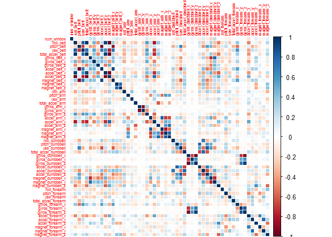
Correlation Matrix of Columns in the Training Data set.
corrplot(cor(training[, -length(names(training))]), method = "color", tl.cex = 0.5)we split the cleaned training set into a pure training data set (70%) and a validation data set (30%). We will use the validation data set to conduct cross validation in future steps.
set.seed(56789) # For reproducibile purpose
inTrain <- createDataPartition(training$classe, p = 0.70, list = FALSE)
validation <- training[-inTrain, ]
training <- training[inTrain, ]
rm(inTrain)
The Dataset now consists of 54 variables with the observations divided as following:
- Training Data: 13737 observations.
- Validation Data: 5885 observations.
- Testing Data: 20 observations.
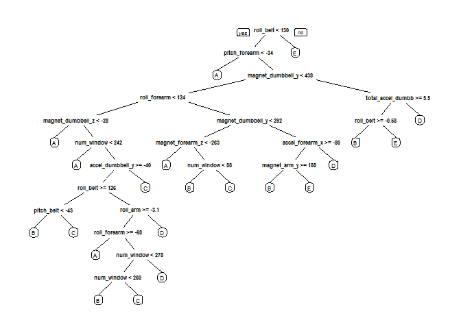
We fit a predictive model for activity recognition using Decision Tree algorithm.
modelTree <- rpart(classe ~ ., data = training, method = "class")
prp(modelTree)
Now, we estimate the performance of the model on the validation data set.
predictTree <- predict(modelTree, validation, type = "class")
confusionMatrix(validation$classe, predictTree)
## Confusion Matrix and Statistics
##
## Reference
## Prediction A B C D E
## A 1526 41 20 61 26
## B 264 646 74 126 29
## C 20 56 852 72 26
## D 93 31 133 665 42
## E 82 85 93 128 694
##
## Overall Statistics
##
## Accuracy : 0.7448
## 95% CI : (0.7334, 0.7559)
## No Information Rate : 0.3373
## P-Value [Acc > NIR] : < 2.2e-16
##
## Kappa : 0.6754
## Mcnemar's Test P-Value : < 2.2e-16
##
## Statistics by Class:
##
## Class: A Class: B Class: C Class: D Class: E
## Sensitivity 0.7688 0.7520 0.7270 0.6321 0.8494
## Specificity 0.9621 0.9019 0.9631 0.9381 0.9234
## Pos Pred Value 0.9116 0.5672 0.8304 0.6898 0.6414
## Neg Pred Value 0.8910 0.9551 0.9341 0.9214 0.9744
## Prevalence 0.3373 0.1460 0.1992 0.1788 0.1388
## Detection Rate 0.2593 0.1098 0.1448 0.1130 0.1179
## Detection Prevalence 0.2845 0.1935 0.1743 0.1638 0.1839
## Balanced Accuracy 0.8654 0.8270 0.8450 0.7851 0.8864
accuracy <- postResample(predictTree, validation$classe)
ose <- 1 - as.numeric(confusionMatrix(validation$classe, predictTree)$overall[1])
rm(predictTree)
rm(modelTree)
The Estimated Accuracy of the Random Forest Model is 74.4774851% and the Estimated Out-of-Sample Error is 25.5225149%.
We fit a predictive model for activity recognition using Random Forest algorithm because it automatically selects important variables and is robust to correlated covariates & outliers in general.
We will use 5-fold cross validation when applying the algorithm.
modelRF <- train(classe ~ ., data = training, method = "rf", trControl = trainControl(method = "cv", 5), ntree = 250)
modelRF
## Random Forest
##
## 13737 samples
## 53 predictor
## 5 classes: 'A', 'B', 'C', 'D', 'E'
##
## No pre-processing
## Resampling: Cross-Validated (5 fold)
##
## Summary of sample sizes: 10989, 10988, 10991, 10990, 10990
##
## Resampling results across tuning parameters:
##
## mtry Accuracy Kappa Accuracy SD Kappa SD
## 2 0.9941762 0.9926331 0.0015235050 0.001927342
## 27 0.9971607 0.9964086 0.0009432244 0.001192905
## 53 0.9948309 0.9934612 0.0018827897 0.002381830
##
## Accuracy was used to select the optimal model using the largest value.
## The final value used for the model was mtry = 27.
Now, we estimate the performance of the model on the validation data set.
predictRF <- predict(modelRF, validation)
confusionMatrix(validation$classe, predictRF)
## Confusion Matrix and Statistics
##
## Reference
## Prediction A B C D E
## A 1674 0 0 0 0
## B 0 1139 0 0 0
## C 0 1 1022 3 0
## D 0 0 2 962 0
## E 0 0 0 1 1081
##
## Overall Statistics
##
## Accuracy : 0.9988
## 95% CI : (0.9976, 0.9995)
## No Information Rate : 0.2845
## P-Value [Acc > NIR] : < 2.2e-16
##
## Kappa : 0.9985
## Mcnemar's Test P-Value : NA
##
## Statistics by Class:
##
## Class: A Class: B Class: C Class: D Class: E
## Sensitivity 1.0000 0.9991 0.9980 0.9959 1.0000
## Specificity 1.0000 1.0000 0.9992 0.9996 0.9998
## Pos Pred Value 1.0000 1.0000 0.9961 0.9979 0.9991
## Neg Pred Value 1.0000 0.9998 0.9996 0.9992 1.0000
## Prevalence 0.2845 0.1937 0.1740 0.1641 0.1837
## Detection Rate 0.2845 0.1935 0.1737 0.1635 0.1837
## Detection Prevalence 0.2845 0.1935 0.1743 0.1638 0.1839
## Balanced Accuracy 1.0000 0.9996 0.9986 0.9977 0.9999
accuracy <- postResample(predictRF, validation$classe)
ose <- 1 - as.numeric(confusionMatrix(validation$classe, predictRF)$overall[1])
rm(predictRF)
The Estimated Accuracy of the Random Forest Model is 99.8810535% and the Estimated Out-of-Sample Error is 0.1189465%.
Random Forests yielded better Results, as expected!
Now, we apply the Random Forest model to the original testing data set downloaded from the data source. We remove the problem_id column first.
rm(accuracy)
rm(ose)
predict(modelRF, testing[, -length(names(testing))])
## [1] B A B A A E D B A A B C B A E E A B B B
## Levels: A B C D E
Function to generate files with predictions to submit for assignment.
pml_write_files = function(x){
  n = length(x)
  for(i in 1:n){
    filename = paste0("./Assignment_Solutions/problem_id_",i,".txt")
    write.table(x[i], file = filename, quote = FALSE, row.names = FALSE, col.names = FALSE)
  }
}
Generating the Files.
pml_write_files(predict(modelRF, testing[, -length(names(testing))]))
rm(modelRF)
rm(training)
rm(testing)
rm(validation)
rm(pml_write_files)
