Louis-Finegan / Convection-Diffusion-Models-Finite-Difference-Method-Python3

Applying the finite-difference method to the Convection Diffusion equation in python3. Examples included: One dimensional Heat equation, Transport equation, Fokker-Plank equation and some two dimensional examples.

Diffusion Convection Equation

Introduction

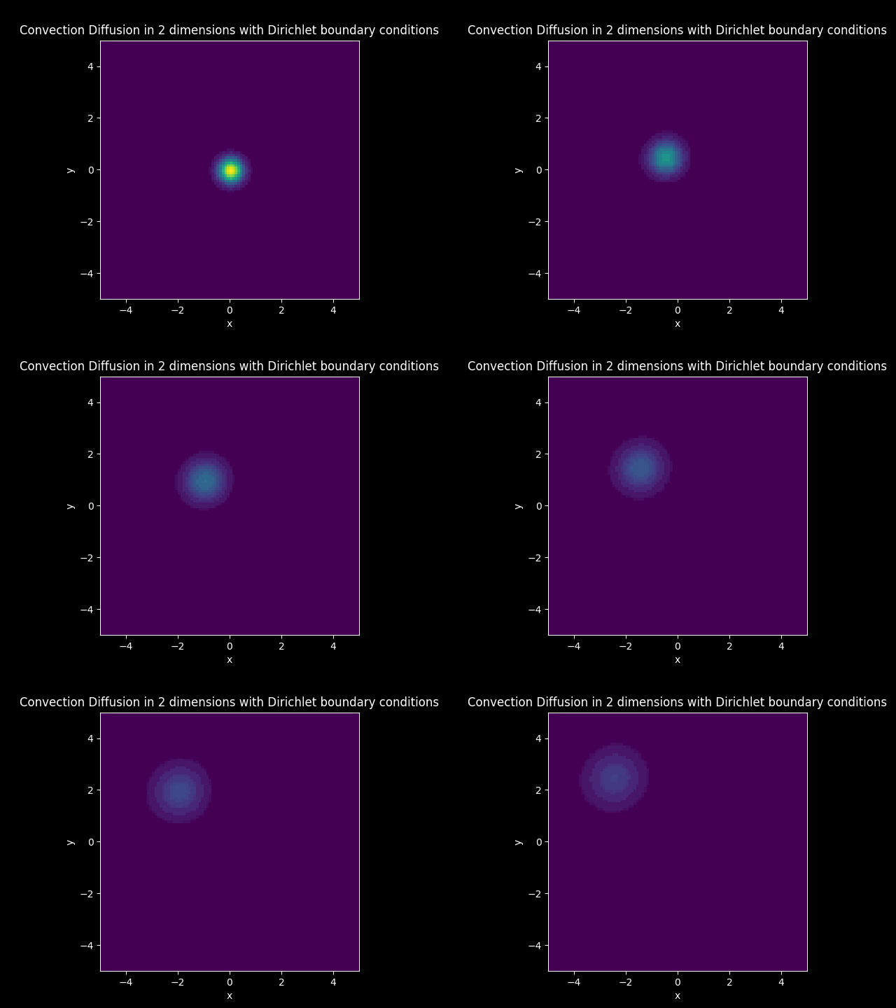
The Diffusion Convection Equation is a Partial Differential Equation writen in the form:

$$\frac{\partial u}{\partial t} = \nabla ( D \nabla u) + \nabla \cdot (\mathbf{c} u)$$

This Equation can model most physical phenomena involving the transfer of a quantity by 'Diffusion' and 'Convection' (Advection).

1. $\nabla(D \nabla u)$ is the diffusion term. Diffusion describes the net movement of a quantity $u$, generally from a region of higher concentration to lower concentraction.

2. $\nabla \cdot (\mathbf{c} u)$ is the convection term. Convection (Advection) describes the bulk motion of a quantity $u$ under the a velocity field $\mathbf{c}$.

Click here for more information on the Diffusion Convection Equation.

Simplifications

There are a number of simplifications made to this model.

1. Let the diffusion coefficient $D$ be constant, this means it can come outside of the gradient operator resulting in the dot product of the gradients becoming the Laplacian. Hence the diffusion is written as $D \nabla^2 u$.

2. Let the convection vector field be constant, this means the convection term siplifies to $\mathbf{c} \cdot \nabla u$.

Diffusion Equation

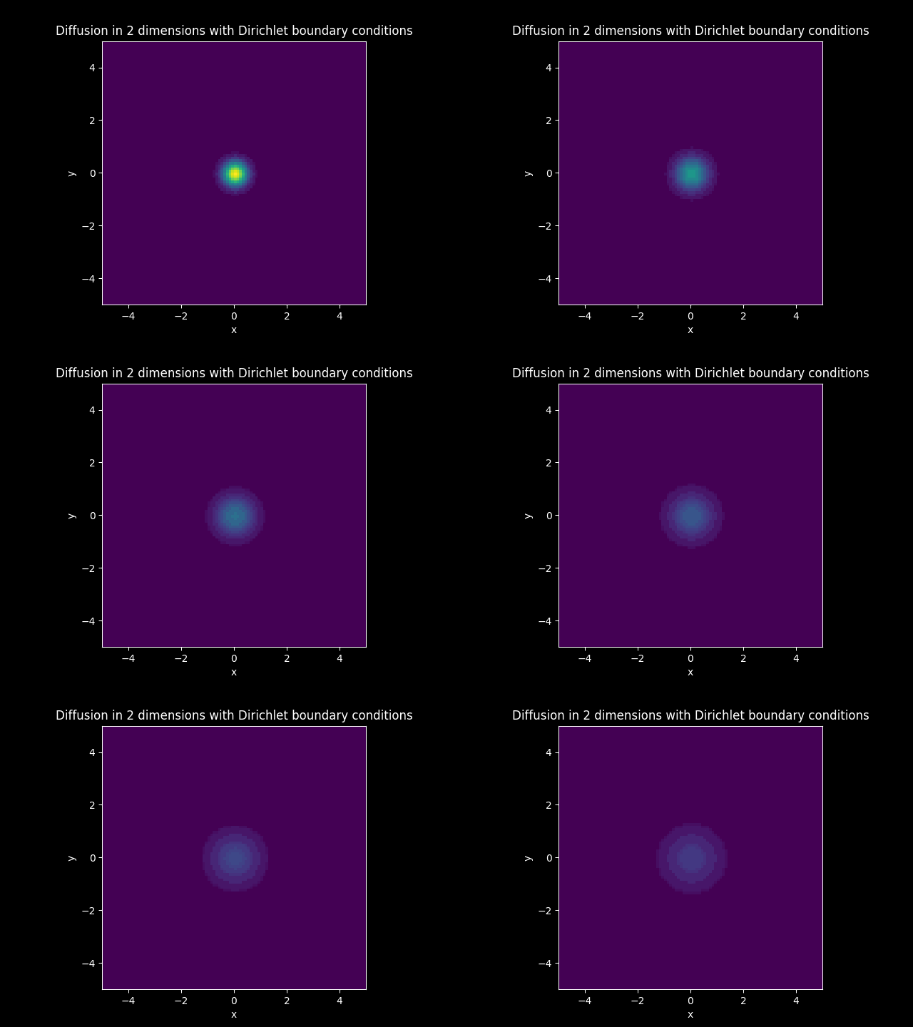
Suppose a model where $\mathbf{c} = 0$. This can be interpreted as a quantity $u$ under going diffusion only, so $u$ is not flowing with any vector field. instead it is moving into the less concentrated areas. This model is governed by the following Partial Differential Equation:

$$\frac{\partial u}{\partial t} = D\nabla^2 u$$

Convection Equation

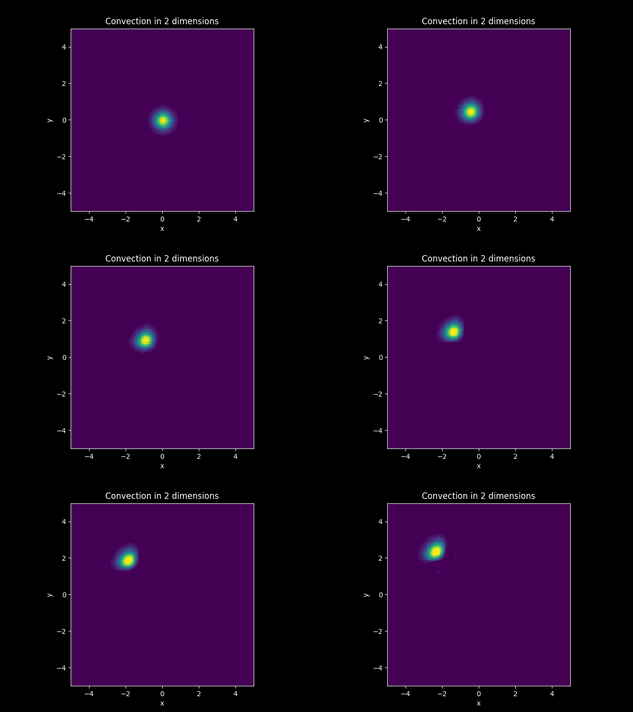
Suppose a model where $D = 0$. this can be interpreted as a under going convection only, so $u$ is being transported with the same density distribution by a constant vector field $\mathbf{c}$. This model is governed by the following Partial Differential Equation:

$$\frac{\partial u}{\partial t} = \mathbf{c} \cdot \nabla u$$

Examples

Consider a Diffusion Convection model in 2 dimension with the vector $\mathbf{c}$ having equal vector components and $D$ is constant.

Let $\mathbf{c} = [-0.1, -0.1]$ and $D = 0.009$. (Neumann boundary condition and 3d animations can be found in Two dimensional examples)

Diffusion Convection Model

Solution:

Diffusion Model

Solution:

Convection Model

Solution:

Applications

Some applications of these models include:

1. Heat Transfer or cooling of a system.

2. Tranportation of a fluids density distribution that is flowing uniformly.

3. Fokker Plank Equation of a Stochastic Differential Equation with uniform drift and standard deviation.