[UNDER DEVELOPMENT]
- 1. Applications of
Machine Learning - 2. Difference between AI, ML and DL
- 3. Data Preprocessing
- 4. Regression
- 5. How to choose the most suitable models
- 6. Classification
Currently, almost everything we use is already using Machine Learning (ML) in some way, for example: whenever you post on Facebook, it already knows who your friends are in the photo and automatically tags them, this implies another application which is Recognition Facial that is being widely adopted. This is an example that almost everyone has seen, but we can mention others, such as: the X-Box Kinect, which analyzes your actions and reproduces them in the game you are playing and the name of the algorithm used in this scenario isc alled the Forest Random, we can also quote Netflix with it's system of recommendations for films and series, which learns from the informations provided, such as the time you spend watching a specific program, which were marked with like or deslike, Virtual Stores also use the Machine Learning to offer new products according to your consumption or visualizations, the keyboard of your SmartPhone learns while you type your messages or surveys, Virtual Reality (VR) glasses, Machine Learning is also use to save lives, helping to detect cancer and making new drugs, vaccines and other things that would take a long time if only humans wre analyzed.
I can cite many other examples, but I suggest paying close attention to the behavior of the tools you use on a daily basis and if you notice that it seems to know you very well or that it makes very accurate predictions, this will probably indicate that this tool is using Machine Learning in some part of it's functioning.
There is often a difficulty in understanding the differences between Artificial Intelligence (AI), Machine Learning (ML) and Deep Learning (DL). Terms that are not recent, but that have gained greater popularity in the last decade.

Artificial Intelligence is a term that was created in 1955 and that can be interpreted basically as the name suggests, that is, the incorporation of human intelligence in machines.
So, whenever a machine performs a task, which has been implemented with a set of instructions (algorithms), we call this "Intelligent" behavior Artificial Intelligence. There we can concluded that all machines that perform some tasks through algorithms are "equipped" with Artificial Intelligence.
If it is still difficult to observe this, we can cite some examples very close to us, such as: our fridges, washing machines, SmartPhones, car or house alarms, among thousands of other devices that we use in our day today.
Again, as the name suggests, it is the ability of machines to learn and we can interpret this as a way of instructing machines with teachings so that they can perform specific tasks.
We can do this by providing data so that the machine understands the patterns (training) and from there makes decisions based on what it has learned. It is like teaching certain taks to a child, you explain to him how to perform a certain task with examples (data), he performs that task several times to really learn (training) and, depending on this performance, you help him so that he can perform the task more efficiently (accurately).
Deep Learning is a subset of the Machine Learning universe, we can interpret it as the next evolution of Machine Learning itself.
DL is inspired by the functioning of the human brain in relation to pattern processing.
Just as our brain identifies patterns and classifies them, Deep Learning algorithms are implemented to behave in the same way.
Comparing the functioning of Deep Learning and Machine Learning, we can see that while the DL can discover the features that must be applied in a classification, the ML needs that these features are provided manually.
In this stage of data Preprocessing, we will start a Notebook with the following approaches:
-
Importing the Libraries
-
Importing the Dataset
-
Taking care of Missing Data:
We perform this procedure by taking the empty data and replacing it with the average.
-
Enconding Categorical Data:
Encoding is necessary at this point, because as there is no relationship between country names, we do not want an incorrect interpretation made by the model, which would causa inaccurate correlattions and consequently impact it's accuracy. So, the encoding methods applied here is One Hot Encoding and to Purchased column we applied the Label Encoding.
For more about encondig methods, see the following link: All about Categorical Variable Encoding
For more about Categorial variable, see the following link: Categorical Variable -
Spliting the dataset into the Training set and Test Set:
In this step, we apply the Feature Scaling after splitting the data set into two other sets, which are: Testing and Training. This is because the Test data set is composed of new data, which has not yet been observed. Therefore, these cannot be mixed with the Training data set.
The use of any data from the Test suite before or during training is a potential bias in assessing performance. -
Feature Scalling:
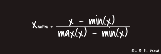
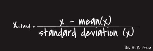
Feature scaling is the process of scaling the values of features in a dataset so that they proportionally contribute to the distance calculation. The two most commonly used feature scaling techniques are Standardisation (or Z-Score Normalisation) and Min-Max scaling.
Normalisation: Is recommended when have a normal distribuition on most of your resources.
Standardisation: We use this approach in most situations, as it always provides good performance towards standard deviation.
References:
Feature Scaling and Normalisation in a nutshell
Euclidian Distance


With so many models available, it is normal ot be in doubt about which to select for each situation. For this, we will use the R² method to evaluate the performance of our model, so we can be sure if we are making the most appropriate choice.
Obs.: To display the Adjusted R in models implemented in R. After executing all the code, execute the summary() command with the variable regressor. Example: summary(regressor)
Click to see the sample image

| Multiple Linear Regression | 🐍 Notebook code |
|---|---|
| Polynomial Linear Regression | 🐍 Notebook code |
| Support Vector Regression (SVR) | 🐍 Notebook code |
| Decision Tree Regression | 🐍 Notebook code |
| Random Forest Regressio | 🐍 Notebook code |
📌 Topics covered:
The coefficient of determination denoted R² and pronounced "R squared", is the proportion of the variance in the dependent variable that is predictable from the independent variable(s).
The R² varies between 0 and 1, sometimes being expressed in percentage terms. In this case, it express the amount of variance in the data that is explained by the linear model. Thus, the higher the R², the more explanatory the linear model is, that is, the better it fits the sample. For example, an R² = 0.8234 means that the linear model explains 82.34% of the variance of the dependent variable from the regressors (independent variables) included in that linear model.
We will use a more efficient version of R², which is the adjusted R². And the reason for this is because by including numerous variables, even though they have very little explanatory power over the dependent variable, they will increase the value of R². This encourages the indiscriminate inclusion of variables, which may increase the R² superficially, with variables that are not relevent to our predictions. To combat this trend, we will use the **adjusted R², which penalizes the inclusion of little explanatory regressors.

- p = where p is the total number of explanatory variables in the model (not including the constant term);
- n = n is the sample size;
References:
Coefficient of determination
Unlike regression where you predict a continuous number, you use classification to predict a category. There is a wide variety of classification applications from medicine to marketing. Classification models include linear models like Logistic Regression, SVM, and nonlinear ones like K-NN, Kernel SVM and Random Forests.
⚠️ Because these algorithms contain many calculations, the execution of these codes can take a few minutes.
📌 Topics covered:
Logistic Regression is a statiscal technique that aims to produce, from a set of observations, a model that allows the prediction of categories, from a series of continuous and/or binary explanatory variables. THis provides a discrete binary outcome between 0 and 1.
In comparison with known regression techniques, especially linear regression, Logistic Regression is essentially distinguished by the fact that the response variable is categorical.
The Logistic Regression uses the Sigmoid Function to create your models and this is a mathematical expansion function used in economics and computing, it has this name because of it's S-shaped curve. It will process any number with real value and map it between 0 and 1.

A measure of the relationship that may exist between the dependent variable (our label/category that you want to predict) is carried out with one or more independent variables(our features). After that, the probability that exists between these relationships is estimated.
SCENARIO:
We will use the following scenario as a basis for the following example:
The company that hired us sends emails with offers to it's customers and wants to know the probability among the age groups that will accept the offers or ignore them.
In order to obtain a Logistic Regression with some characteristics of linear regression but with the S-shaped curve of the Sigmoid Function, we need to apply the following equation, which is the junction of the Sigmoid Function with the linear regression equation.

After that, we can see how the probabilities are obtained, this is called p_hat (p^). These probabilities are related to the percentage of chance that exists for a certain age group and would accept the offer sent via email or not.

Finally, we bneed to obtain the value of our prediction, which is related to our dependent value (DV), but since we want the prediction to be not the real value of the probability, we will be call this representation of the result of y as y_hat (y^), which, the results will be displayed by 0 or 1.

- In medicine, it allows for example to determine the factors that characterize a group of sick individuals in relation to healthy individuals;
- In the insurance field, it allows us to find fractions of the clientele that are sensitive to a certain insurance policy in relation to a given particular risk;
- In financial institutions, it can detect risk groups for underwriting credit;
- Predict whether a voter will vote for a given party based on age, income, sex, race, state of residence, votes in previous elections, etc. of the voter;
- It can also be used in engineering, especially to predict the probability of failure in a given process, system, or product;
- Can be used to predict the risk of developing a given disease (for example, diabetes or coronary artery disease), based on the patient's observed characteristics (age, sex, body mass index, results of various blood tests, etc.).
⚠️ This is a brief outline of that is behind the Logistic Regression, it is always good to study a little more about the functioning of this classification model. See the references.
References:
Logistic regression
Sigmoid Function
⚠️ Because these algorithms contain many calculations, the execution of these codes can take a few minutes.
📌 Topics covered:
KNN (K - closest neighbors) is a supervised learning algorithm that can be applied in classification or regression.
K-NN is a type of instance-based (means that our algorithm doesn't explicity learn a model. Instead, it chooses to memorize the training instances) learning, or slow learning, in which the function is approximated only locally. Since this algorithm depends on the distance to be classified, normalizing the training data can dramatically improve its accuracy.
In the graph below we show a situation in which we want classify the gray point in class A or class B.

From this, the calculation of the distance between the gray point and it's K-Nearest points is started.

Step 1: Choose the number K of neighbors;
Step 2: Take the K nearest neighbors of the new data point, according to the Euclidian distance;
Step 3: Among these K neighbors, count the number of data points in each category;
Step 4: Assign the new data point to the category where you counted the most nighbors.
Euclidean distance is usually the most used method to determine the distance between the point we want to include and its neighbors.

However, there are other approaches, as we can see below:
References:
K-Nearest Neighbors algorithm
Hamming Distance
What is Hamming Distance?
Taxicab geometry (Manhattan Distance)
Minkowski distance
⚠️ Because these algorithms contain many calculations, the execution of these codes can take a few minutes.
We already covered this algorithm in the Regression section, so for more details, access this section. However, as we will se below, we will briefly explain the behavior of SVM in the Classification environment.
📌 Topics covered:
As we have already seen in Regression section, the SVM works with a line that divides the data, that line is called a Hyperplane and in the case of classification, we want to find the best way to position this line, which will eventually assign to which class the to which class the new data will be added.

Then, the line is determined by the maximum margin between the classes of points. The distance between the point and the line (hyperplane) is equidistant, that is, the distance from the point close to the margin to the hyperplane, is equivalent for both sides.

And the name of Support Vector comes from those two points flagged below, which basically support the entire algorithm. So, even if you get rid of all the remaining points, the algorithm will be exactly the same.

Next, we can see the hyperplane, which is also known as the maximum margin classifier. For more details, look at how it is described in the Regression section

Finally, we have the lines that represent the margins and these can be called here in our case as Positive Hyperplane and Negative Hyperplane, but as this is just a way of labeling the categories of the classes, we could simply call it a red category or a green category.

⚠️ This is a brief outline of that is behind the Support Vector Machine, it is always good to study a little more about the functioning of this classification model. See the references and Regression section (SVM).
References:
Equidistant